


注意
跳轉到末尾 下載完整的示例程式碼。
簡介 || 張量 || 自動微分 || 構建模型 || TensorBoard 支援 || 訓練模型 || 模型理解
PyTorch 入門#
創建於:2021年11月30日 | 最後更新:2025年6月5日 | 最後驗證:2024年11月5日
請觀看下面的影片或在 youtube 上觀看。
PyTorch 張量#
請觀看影片中從 03:50 開始的部分。
首先,我們將匯入 PyTorch。
import torch
讓我們看看一些基本的張量操作。首先,介紹幾種建立張量的方法。
z = torch.zeros(5, 3)
print(z)
print(z.dtype)
tensor([[0., 0., 0.],
        [0., 0., 0.],
        [0., 0., 0.],
        [0., 0., 0.],
        [0., 0., 0.]])
torch.float32
上面,我們建立了一個 5x3 的全零矩陣,並查詢了其資料型別,發現這些零是 32 位浮點數,這是 PyTorch 的預設型別。
如果你想要整數怎麼辦?你可以隨時覆蓋預設值。
i = torch.ones((5, 3), dtype=torch.int16)
print(i)
tensor([[1, 1, 1],
        [1, 1, 1],
        [1, 1, 1],
        [1, 1, 1],
        [1, 1, 1]], dtype=torch.int16)
你可以看到,當我們改變預設值時,張量在列印時會很友好地報告這一點。
通常,我們會隨機初始化學習權重,並經常設定一個特定的 PRNG 種子以保證結果的可復現性。
torch.manual_seed(1729)
r1 = torch.rand(2, 2)
print('A random tensor:')
print(r1)

r2 = torch.rand(2, 2)
print('\nA different random tensor:')
print(r2) # new values

torch.manual_seed(1729)
r3 = torch.rand(2, 2)
print('\nShould match r1:')
print(r3) # repeats values of r1 because of re-seed
A random tensor:
tensor([[0.3126, 0.3791],
        [0.3087, 0.0736]])

A different random tensor:
tensor([[0.4216, 0.0691],
        [0.2332, 0.4047]])

Should match r1:
tensor([[0.3126, 0.3791],
        [0.3087, 0.0736]])
PyTorch 張量進行算術運算非常直觀。形狀相似的張量可以相加、相乘等。與標量的運算會分散到整個張量中。
ones = torch.ones(2, 3)
print(ones)

twos = torch.ones(2, 3) * 2 # every element is multiplied by 2
print(twos)

threes = ones + twos       # addition allowed because shapes are similar
print(threes)              # tensors are added element-wise
print(threes.shape)        # this has the same dimensions as input tensors

r1 = torch.rand(2, 3)
r2 = torch.rand(3, 2)
# uncomment this line to get a runtime error
# r3 = r1 + r2
tensor([[1., 1., 1.],
        [1., 1., 1.]])
tensor([[2., 2., 2.],
        [2., 2., 2.]])
tensor([[3., 3., 3.],
        [3., 3., 3.]])
torch.Size([2, 3])
這裡是可用數學運算的一個小樣本。
r = (torch.rand(2, 2) - 0.5) * 2 # values between -1 and 1
print('A random matrix, r:')
print(r)

# Common mathematical operations are supported:
print('\nAbsolute value of r:')
print(torch.abs(r))

# ...as are trigonometric functions:
print('\nInverse sine of r:')
print(torch.asin(r))

# ...and linear algebra operations like determinant and singular value decomposition
print('\nDeterminant of r:')
print(torch.det(r))
print('\nSingular value decomposition of r:')
print(torch.svd(r))

# ...and statistical and aggregate operations:
print('\nAverage and standard deviation of r:')
print(torch.std_mean(r))
print('\nMaximum value of r:')
print(torch.max(r))
A random matrix, r:
tensor([[ 0.9956, -0.2232],
        [ 0.3858, -0.6593]])

Absolute value of r:
tensor([[0.9956, 0.2232],
        [0.3858, 0.6593]])

Inverse sine of r:
tensor([[ 1.4775, -0.2251],
        [ 0.3961, -0.7199]])

Determinant of r:
tensor(-0.5703)

Singular value decomposition of r:
torch.return_types.svd(
U=tensor([[-0.8353, -0.5497],
        [-0.5497,  0.8353]]),
S=tensor([1.1793, 0.4836]),
V=tensor([[-0.8851, -0.4654],
        [ 0.4654, -0.8851]]))

Average and standard deviation of r:
(tensor(0.7217), tensor(0.1247))

Maximum value of r:
tensor(0.9956)
關於 PyTorch 張量的強大功能還有更多內容需要了解,包括如何設定它們進行 GPU 平行計算——我們將在另一個影片中進行更深入的探討。
PyTorch 模型#
請觀看影片中從 10:00 開始的部分。
讓我們來談談如何在 PyTorch 中表達模型。
import torch                     # for all things PyTorch
import torch.nn as nn            # for torch.nn.Module, the parent object for PyTorch models
import torch.nn.functional as F  # for the activation function
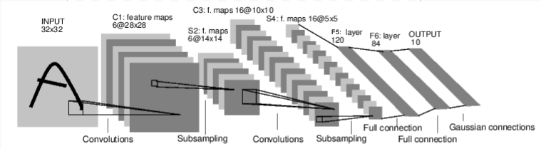
圖:LeNet-5
上面是 LeNet-5 的圖示,它是最早的卷積神經網路之一,也是深度學習爆炸式發展的驅動力之一。它被構建用於讀取手寫數字的小影像(MNIST 資料集),並正確地將影像中表示的數字分類。
以下是其工作原理的簡化版本。
C1 層是一個卷積層,意味著它會在輸入影像中掃描在訓練期間學習到的特徵。它會輸出一個圖,顯示它在影像中看到每個學習到的特徵的位置。這個“啟用圖”在 S2 層被下采樣。
C3 層是另一個卷積層,這次它會掃描 C1 的啟用圖來尋找特徵的 *組合*。它還會輸出一個啟用圖,描述這些特徵組合的空間位置,這個圖在 S4 層被下采樣。
最後,末尾的全連線層 F5、F6 和 OUTPUT 是一個 *分類器*,它接收最終的啟用圖,並將其分類到代表 10 個數字的 10 個 bin 中。
我們如何在程式碼中表達這個簡單的神經網路?
class LeNet(nn.Module):

    def __init__(self):
        super(LeNet, self).__init__()
        # 1 input image channel (black & white), 6 output channels, 5x5 square convolution
        # kernel
        self.conv1 = nn.Conv2d(1, 6, 5)
        self.conv2 = nn.Conv2d(6, 16, 5)
        # an affine operation: y = Wx + b
        self.fc1 = nn.Linear(16 * 5 * 5, 120)  # 5*5 from image dimension
        self.fc2 = nn.Linear(120, 84)
        self.fc3 = nn.Linear(84, 10)

    def forward(self, x):
        # Max pooling over a (2, 2) window
        x = F.max_pool2d(F.relu(self.conv1(x)), (2, 2))
        # If the size is a square you can only specify a single number
        x = F.max_pool2d(F.relu(self.conv2(x)), 2)
        x = x.view(-1, self.num_flat_features(x))
        x = F.relu(self.fc1(x))
        x = F.relu(self.fc2(x))
        x = self.fc3(x)
        return x

    def num_flat_features(self, x):
        size = x.size()[1:]  # all dimensions except the batch dimension
        num_features = 1
        for s in size:
            num_features *= s
        return num_features
檢視上面的程式碼,你應該能發現與上述圖示的一些結構相似之處。
這演示了一個典型 PyTorch 模型的結構。
它繼承自
torch.nn.Module——模組可以巢狀——事實上,即使是Conv2d和Linear層類也繼承自torch.nn.Module。模型將有一個
__init__()函式,在其中它例項化其層,並載入任何可能需要的 資料工件(例如,NLP 模型可能會載入詞彙表)。模型將有一個
forward()函式。這是實際發生計算的地方:輸入透過網路層和各種函式生成輸出。除此之外,你可以像其他 Python 類一樣構建你的模型類,新增任何你需要支援模型計算的屬性和方法。
讓我們例項化這個物件,並執行一個樣本輸入。
net = LeNet()
print(net)                         # what does the object tell us about itself?

input = torch.rand(1, 1, 32, 32)   # stand-in for a 32x32 black & white image
print('\nImage batch shape:')
print(input.shape)

output = net(input)                # we don't call forward() directly
print('\nRaw output:')
print(output)
print(output.shape)
LeNet(
  (conv1): Conv2d(1, 6, kernel_size=(5, 5), stride=(1, 1))
  (conv2): Conv2d(6, 16, kernel_size=(5, 5), stride=(1, 1))
  (fc1): Linear(in_features=400, out_features=120, bias=True)
  (fc2): Linear(in_features=120, out_features=84, bias=True)
  (fc3): Linear(in_features=84, out_features=10, bias=True)
)

Image batch shape:
torch.Size([1, 1, 32, 32])

Raw output:
tensor([[ 0.0898,  0.0318,  0.1485,  0.0301, -0.0085, -0.1135, -0.0296,  0.0164,
          0.0039,  0.0616]], grad_fn=<AddmmBackward0>)
torch.Size([1, 10])
上面有幾件重要的事情正在發生。
首先,我們例項化 LeNet 類,並列印 net 物件。 torch.nn.Module 的一個子類會報告它建立的層及其形狀和引數。如果你想了解模型處理過程的梗概,這可以提供一個方便的概述。
在此下方,我們建立一個代表 32x32 影像(1 個顏色通道)的虛擬輸入。通常,你會載入一個影像塊並將其轉換為此形狀的張量。
你可能注意到了我們張量中多了一個維度——*批次維度*。PyTorch 模型假定它們處理的是資料 *批次*——例如,16 個我們的影像塊的批次將具有形狀 (16, 1, 32, 32)。由於我們只使用一張影像,因此我們建立了一個批次大小為 1 的批次,形狀為 (1, 1, 32, 32)。
我們透過像呼叫函式一樣呼叫模型來請求推理:net(input)。此呼叫的輸出代表模型對輸入表示特定數字的置信度。(由於此模型例項尚未學習任何內容,因此我們不應期望在輸出中看到任何訊號。)檢視 output 的形狀,我們可以看到它也有一個批次維度,其大小應始終與輸入批次維度匹配。如果我們傳入一個 16 個例項的輸入批次,output 的形狀將是 (16, 10)。
資料集和資料載入器#
請觀看影片中從 14:00 開始的部分。
下面,我們將演示如何使用 TorchVision 中一個可直接下載的、公開訪問的資料集,如何轉換影像以供模型使用,以及如何使用 DataLoader 將資料批次饋送給模型。
我們需要做的第一件事是將輸入的影像轉換為 PyTorch 張量。
#%matplotlib inline

import torch
import torchvision
import torchvision.transforms as transforms

transform = transforms.Compose(
    [transforms.ToTensor(),
     transforms.Normalize((0.4914, 0.4822, 0.4465), (0.2470, 0.2435, 0.2616))])
在這裡,我們為輸入指定了兩個轉換。
transforms.ToTensor()將 Pillow 載入的影像轉換為 PyTorch 張量。transforms.Normalize()調整張量的值,使其平均值為零,標準差為 1.0。大多數啟用函式在 x = 0 附近具有最強的梯度,因此將資料集中在此可以加快學習速度。傳遞給變換的值是資料集中影像 RGB 值的均值(第一個元組)和標準差(第二個元組)。你可以透過執行以下幾行程式碼自己計算這些值。from torch.utils.data import ConcatDataset transform = transforms.Compose([transforms.ToTensor()]) trainset = torchvision.datasets.CIFAR10(root='./data', train=True, download=True, transform=transform) # stack all train images together into a tensor of shape # (50000, 3, 32, 32) x = torch.stack([sample[0] for sample in ConcatDataset([trainset])]) # get the mean of each channel mean = torch.mean(x, dim=(0,2,3)) # tensor([0.4914, 0.4822, 0.4465]) std = torch.std(x, dim=(0,2,3)) # tensor([0.2470, 0.2435, 0.2616])
有更多可用的變換,包括裁剪、居中、旋轉和翻轉。
接下來,我們將建立一個 CIFAR10 資料集的例項。這是一個由 32x32 顏色影像塊組成的集合,代表 10 類物件:6 種動物(鳥、貓、鹿、狗、青蛙、馬)和 4 種車輛(飛機、汽車、船、卡車)。
trainset = torchvision.datasets.CIFAR10(root='./data', train=True,
                                        download=True, transform=transform)
  0%|          | 0.00/170M [00:00<?, ?B/s]
  0%|          | 459k/170M [00:00<00:37, 4.51MB/s]
  3%|▎         | 5.51M/170M [00:00<00:05, 31.3MB/s]
  7%|▋         | 11.4M/170M [00:00<00:03, 44.0MB/s]
 11%|█         | 18.6M/170M [00:00<00:02, 54.7MB/s]
 15%|█▍        | 25.5M/170M [00:00<00:02, 59.7MB/s]
 19%|█▉        | 32.7M/170M [00:00<00:02, 63.8MB/s]
 23%|██▎       | 40.0M/170M [00:00<00:01, 66.8MB/s]
 28%|██▊       | 47.0M/170M [00:00<00:01, 67.8MB/s]
 32%|███▏      | 54.2M/170M [00:00<00:01, 69.1MB/s]
 36%|███▌      | 61.4M/170M [00:01<00:01, 70.0MB/s]
 40%|████      | 68.6M/170M [00:01<00:01, 70.6MB/s]
 45%|████▍     | 75.9M/170M [00:01<00:01, 71.2MB/s]
 49%|████▊     | 83.1M/170M [00:01<00:01, 70.9MB/s]
 53%|█████▎    | 90.5M/170M [00:01<00:01, 71.7MB/s]
 57%|█████▋    | 97.6M/170M [00:01<00:01, 70.9MB/s]
 62%|██████▏   | 105M/170M [00:01<00:00, 71.5MB/s]
 66%|██████▌   | 112M/170M [00:01<00:00, 70.5MB/s]
 70%|███████   | 119M/170M [00:01<00:00, 71.1MB/s]
 74%|███████▍  | 127M/170M [00:01<00:00, 70.5MB/s]
 78%|███████▊  | 134M/170M [00:02<00:00, 70.1MB/s]
 83%|████████▎ | 141M/170M [00:02<00:00, 68.3MB/s]
 87%|████████▋ | 148M/170M [00:02<00:00, 67.0MB/s]
 91%|█████████ | 155M/170M [00:02<00:00, 67.8MB/s]
 95%|█████████▍| 161M/170M [00:02<00:00, 66.7MB/s]
 99%|█████████▊| 168M/170M [00:02<00:00, 66.7MB/s]
100%|██████████| 170M/170M [00:02<00:00, 66.1MB/s]
注意
執行上面的單元格時,資料集下載可能需要一點時間。
這是一個在 PyTorch 中建立資料集物件的示例。可下載的資料集(如上面的 CIFAR-10)是 torch.utils.data.Dataset 的子類。Dataset 類包括 TorchVision、Torchtext 和 TorchAudio 中的可下載資料集,以及像 torchvision.datasets.ImageFolder 這樣的實用資料集類,它會讀取一個包含已標記影像的資料夾。你也可以建立自己的 Dataset 子類。
當我們例項化我們的資料集時,我們需要告訴它一些事情。
資料要存放的檔案的系統路徑。
我們是否正在使用此集合進行訓練;大多數資料集將分為訓練集和測試集。
如果我們還沒有下載資料集,是否希望下載它。
我們想要應用於資料的變換。
一旦你的資料集準備就緒,你就可以將其交給 DataLoader。
trainloader = torch.utils.data.DataLoader(trainset, batch_size=4,
                                          shuffle=True, num_workers=2)
Dataset 子類封裝了對資料的訪問,並且是服務於其資料型別的專業化。 DataLoader 對資料一無所知,但會根據你指定的引數將 Dataset 提供的輸入張量組織成批次。
在上面的示例中,我們要求 DataLoader 從 trainset 提供 4 張影像的批次,隨機化它們的順序(shuffle=True),並告訴它啟動兩個工作程序從磁碟載入資料。
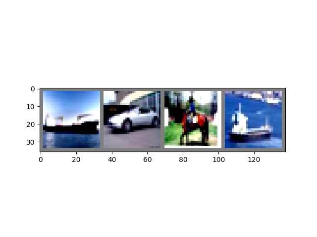
最好視覺化你的 DataLoader 提供的批次。
import matplotlib.pyplot as plt
import numpy as np

classes = ('plane', 'car', 'bird', 'cat',
           'deer', 'dog', 'frog', 'horse', 'ship', 'truck')

def imshow(img):
    img = img / 2 + 0.5     # unnormalize
    npimg = img.numpy()
    plt.imshow(np.transpose(npimg, (1, 2, 0)))


# get some random training images
dataiter = iter(trainloader)
images, labels = next(dataiter)

# show images
imshow(torchvision.utils.make_grid(images))
# print labels
print(' '.join('%5s' % classes[labels[j]] for j in range(4)))
Clipping input data to the valid range for imshow with RGB data ([0..1] for floats or [0..255] for integers). Got range [-0.49473685..1.5632443].
 ship   car horse  ship
執行上面的單元格應該會顯示一個包含四張影像的條帶,以及每張影像的正確標籤。
訓練你的 PyTorch 模型#
請觀看影片中從 17:10 開始的部分。
讓我們把所有部分組合起來,訓練一個模型。
#%matplotlib inline

import torch
import torch.nn as nn
import torch.nn.functional as F
import torch.optim as optim

import torchvision
import torchvision.transforms as transforms

import matplotlib
import matplotlib.pyplot as plt
import numpy as np
首先,我們需要訓練集和測試集。如果你還沒有,請執行下面的單元格以確保資料集已下載。(可能需要一分鐘。)
transform = transforms.Compose(
    [transforms.ToTensor(),
     transforms.Normalize((0.5, 0.5, 0.5), (0.5, 0.5, 0.5))])

trainset = torchvision.datasets.CIFAR10(root='./data', train=True,
                                        download=True, transform=transform)
trainloader = torch.utils.data.DataLoader(trainset, batch_size=4,
                                          shuffle=True, num_workers=2)

testset = torchvision.datasets.CIFAR10(root='./data', train=False,
                                       download=True, transform=transform)
testloader = torch.utils.data.DataLoader(testset, batch_size=4,
                                         shuffle=False, num_workers=2)

classes = ('plane', 'car', 'bird', 'cat',
           'deer', 'dog', 'frog', 'horse', 'ship', 'truck')
我們將對來自 DataLoader 的輸出進行檢查。
import matplotlib.pyplot as plt
import numpy as np

# functions to show an image


def imshow(img):
    img = img / 2 + 0.5     # unnormalize
    npimg = img.numpy()
    plt.imshow(np.transpose(npimg, (1, 2, 0)))


# get some random training images
dataiter = iter(trainloader)
images, labels = next(dataiter)

# show images
imshow(torchvision.utils.make_grid(images))
# print labels
print(' '.join('%5s' % classes[labels[j]] for j in range(4)))
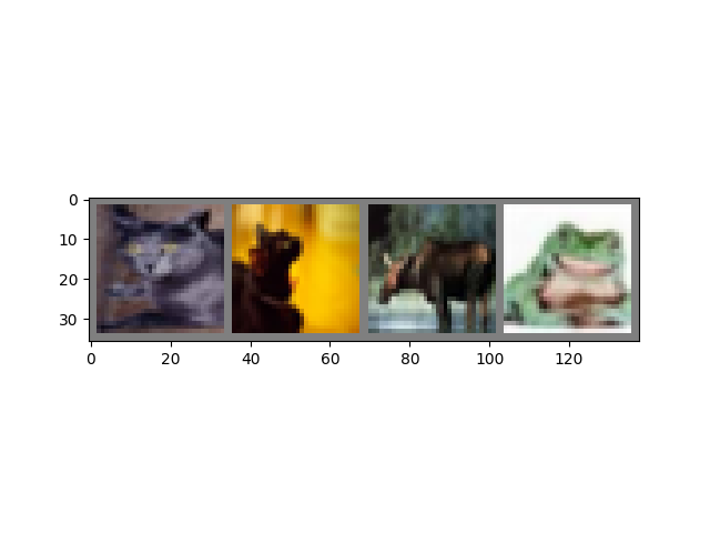
cat cat deer frog
這就是我們將要訓練的模型。如果它看起來很熟悉,那是因為它是 LeNet 的一個變體——在本影片稍早討論過——它被改編用於 3 色影像。
class Net(nn.Module):
    def __init__(self):
        super(Net, self).__init__()
        self.conv1 = nn.Conv2d(3, 6, 5)
        self.pool = nn.MaxPool2d(2, 2)
        self.conv2 = nn.Conv2d(6, 16, 5)
        self.fc1 = nn.Linear(16 * 5 * 5, 120)
        self.fc2 = nn.Linear(120, 84)
        self.fc3 = nn.Linear(84, 10)

    def forward(self, x):
        x = self.pool(F.relu(self.conv1(x)))
        x = self.pool(F.relu(self.conv2(x)))
        x = x.view(-1, 16 * 5 * 5)
        x = F.relu(self.fc1(x))
        x = F.relu(self.fc2(x))
        x = self.fc3(x)
        return x


net = Net()
我們需要的最後一些配料是一個損失函式和一個最佳化器。
criterion = nn.CrossEntropyLoss()
optimizer = optim.SGD(net.parameters(), lr=0.001, momentum=0.9)
損失函式,正如本影片前面討論過的,是我們模型預測與理想輸出之間差距的度量。交叉熵損失是我們這樣的分類模型的典型損失函式。
最佳化器 是驅動學習的機制。在這裡,我們建立了一個實現了*隨機梯度下降*的最佳化器,這是更直接的最佳化演算法之一。除了演算法的引數,如學習率(lr)和動量,我們還傳入了 net.parameters(),這是一個模型中所有學習權重的集合——也就是最佳化器調整的內容。
最後,所有這些都被組裝到訓練迴圈中。繼續執行這個單元格,因為它可能需要幾分鐘才能執行。
for epoch in range(2):  # loop over the dataset multiple times

    running_loss = 0.0
    for i, data in enumerate(trainloader, 0):
        # get the inputs
        inputs, labels = data

        # zero the parameter gradients
        optimizer.zero_grad()

        # forward + backward + optimize
        outputs = net(inputs)
        loss = criterion(outputs, labels)
        loss.backward()
        optimizer.step()

        # print statistics
        running_loss += loss.item()
        if i % 2000 == 1999:    # print every 2000 mini-batches
            print('[%d, %5d] loss: %.3f' %
                  (epoch + 1, i + 1, running_loss / 2000))
            running_loss = 0.0

print('Finished Training')
[1,  2000] loss: 2.195
[1,  4000] loss: 1.879
[1,  6000] loss: 1.656
[1,  8000] loss: 1.576
[1, 10000] loss: 1.517
[1, 12000] loss: 1.461
[2,  2000] loss: 1.415
[2,  4000] loss: 1.368
[2,  6000] loss: 1.334
[2,  8000] loss: 1.327
[2, 10000] loss: 1.318
[2, 12000] loss: 1.261
Finished Training
在這裡,我們只進行了 **2 個訓練週期**(第 1 行)——也就是說,兩次遍歷訓練資料集。每次遍歷都有一個內部迴圈,該迴圈 **迭代訓練資料**(第 4 行),提供轉換後的輸入影像及其正確標籤的批次。
清零梯度(第 9 行)是一個重要的步驟。梯度會在一個批次上累積;如果我們不為每個批次重置它們,它們將繼續累積,這將提供不正確的梯度值,使學習成為不可能。
在第 12 行,我們 **請求模型進行預測**。在下一行(第 13 行),我們計算損失——outputs(模型預測)和 labels(正確輸出)之間的差異。
在第 14 行,我們進行 backward() 傳播,並計算將指導學習的梯度。
在第 15 行,最佳化器執行一個學習步驟——它使用 backward() 呼叫中的梯度來微調學習權重,以它認為會減少損失的方向。
迴圈的其餘部分對週期數、已完成的訓練例項數以及訓練迴圈中累積的損失進行一些簡單的報告。
當你執行上面的單元格時, 你應該會看到類似這樣的內容。
[1,  2000] loss: 2.235
[1,  4000] loss: 1.940
[1,  6000] loss: 1.713
[1,  8000] loss: 1.573
[1, 10000] loss: 1.507
[1, 12000] loss: 1.442
[2,  2000] loss: 1.378
[2,  4000] loss: 1.364
[2,  6000] loss: 1.349
[2,  8000] loss: 1.319
[2, 10000] loss: 1.284
[2, 12000] loss: 1.267
Finished Training
請注意,損失是單調下降的,這表明我們的模型在訓練資料集上的效能持續提高。
作為最後一步,我們應該檢查模型是否真的在進行*通用*學習,而不僅僅是“記憶”資料集。這稱為**過擬合**,通常表明資料集太小(沒有足夠的示例進行通用學習),或者模型具有比其建模資料集所需的更多的學習引數。
這就是為什麼資料集要分成訓練集和測試集——為了測試模型的通用性,我們要求它對未訓練過的資料進行預測。
correct = 0
total = 0
with torch.no_grad():
    for data in testloader:
        images, labels = data
        outputs = net(images)
        _, predicted = torch.max(outputs.data, 1)
        total += labels.size(0)
        correct += (predicted == labels).sum().item()

print('Accuracy of the network on the 10000 test images: %d %%' % (
    100 * correct / total))
Accuracy of the network on the 10000 test images: 54 %
如果你跟著做,你應該看到模型在這個時候大約有 50% 的準確率。這不算是最頂尖的水平,但比我們從隨機輸出預期的 10% 準確率要好得多。這表明模型確實發生了一些通用學習。
指令碼總執行時間: (1 分鐘 23.560 秒)
