


注意
轉到末尾 下載完整的示例程式碼。
計算機視覺遷移學習教程#
建立日期: 2017 年 3 月 24 日 | 最後更新: 2025 年 1 月 27 日 | 最後驗證: 2024 年 11 月 5 日
在本教程中,您將學習如何使用遷移學習來訓練用於影像分類的卷積神經網路。您可以在 cs231n 筆記 中閱讀更多關於遷移學習的內容。
引用這些筆記,
實際上,很少有人從頭開始訓練整個卷積網路(使用隨機初始化),因為擁有足夠大的資料集相對罕見。相反,通常的做法是在非常大的資料集(例如 ImageNet,包含 120 萬張影像和 1000 個類別)上預訓練一個卷積網路,然後將該卷積網路用作初始化或固定的特徵提取器來處理感興趣的任務。
這兩種主要的遷移學習場景如下所示:
微調卷積網路:我們不使用隨機初始化,而是用預訓練網路(例如在 ImageNet 1000 資料集上訓練的網路)初始化網路。其餘的訓練過程照常進行。
將卷積網路作為固定的特徵提取器:在這裡,我們將凍結網路中除最後一個全連線層之外的所有層的權重。最後一個全連線層被一個新的具有隨機權重的層替換,並且只有這一層被訓練。
# License: BSD
# Author: Sasank Chilamkurthy

import torch
import torch.nn as nn
import torch.optim as optim
from torch.optim import lr_scheduler
import torch.backends.cudnn as cudnn
import numpy as np
import torchvision
from torchvision import datasets, models, transforms
import matplotlib.pyplot as plt
import time
import os
from PIL import Image
from tempfile import TemporaryDirectory

cudnn.benchmark = True
plt.ion()   # interactive mode
<contextlib.ExitStack object at 0x7f33e6095150>
載入資料#
我們將使用 torchvision 和 torch.utils.data 包來載入資料。
今天我們要解決的問題是訓練一個模型來分類螞蟻和蜜蜂。我們有大約 120 張螞蟻和蜜蜂的訓練影像。每種類別有 75 張驗證影像。通常,如果從頭開始訓練,這個資料集太小,無法進行泛化。由於我們正在使用遷移學習,我們應該能夠進行相當好的泛化。
該資料集是 ImageNet 的一個非常小的子集。
注意
從 這裡 下載資料,並將其解壓到當前目錄。
# Data augmentation and normalization for training
# Just normalization for validation
data_transforms = {
    'train': transforms.Compose([
        transforms.RandomResizedCrop(224),
        transforms.RandomHorizontalFlip(),
        transforms.ToTensor(),
        transforms.Normalize([0.485, 0.456, 0.406], [0.229, 0.224, 0.225])
    ]),
    'val': transforms.Compose([
        transforms.Resize(256),
        transforms.CenterCrop(224),
        transforms.ToTensor(),
        transforms.Normalize([0.485, 0.456, 0.406], [0.229, 0.224, 0.225])
    ]),
}

data_dir = 'data/hymenoptera_data'
image_datasets = {x: datasets.ImageFolder(os.path.join(data_dir, x),
                                          data_transforms[x])
                  for x in ['train', 'val']}
dataloaders = {x: torch.utils.data.DataLoader(image_datasets[x], batch_size=4,
                                             shuffle=True, num_workers=4)
              for x in ['train', 'val']}
dataset_sizes = {x: len(image_datasets[x]) for x in ['train', 'val']}
class_names = image_datasets['train'].classes

# We want to be able to train our model on an `accelerator <https://pytorch.com.tw/docs/stable/torch.html#accelerators>`__
# such as CUDA, MPS, MTIA, or XPU. If the current accelerator is available, we will use it. Otherwise, we use the CPU.

device = torch.accelerator.current_accelerator().type if torch.accelerator.is_available() else "cpu"
print(f"Using {device} device")
Using cuda device
視覺化幾張圖片#
讓我們視覺化幾張訓練影像,以便了解資料增強。
def imshow(inp, title=None):
    """Display image for Tensor."""
    inp = inp.numpy().transpose((1, 2, 0))
    mean = np.array([0.485, 0.456, 0.406])
    std = np.array([0.229, 0.224, 0.225])
    inp = std * inp + mean
    inp = np.clip(inp, 0, 1)
    plt.imshow(inp)
    if title is not None:
        plt.title(title)
    plt.pause(0.001)  # pause a bit so that plots are updated


# Get a batch of training data
inputs, classes = next(iter(dataloaders['train']))

# Make a grid from batch
out = torchvision.utils.make_grid(inputs)

imshow(out, title=[class_names[x] for x in classes])
![['ants', 'ants', 'bees', 'ants']](../_images/sphx_glr_transfer_learning_tutorial_001.png)
訓練模型#
現在,讓我們編寫一個通用的函式來訓練模型。在這裡,我們將演示
學習率排程
儲存最佳模型
在接下來的內容中,引數 scheduler 是來自 torch.optim.lr_scheduler 的 LR 排程器物件。
def train_model(model, criterion, optimizer, scheduler, num_epochs=25):
    since = time.time()

    # Create a temporary directory to save training checkpoints
    with TemporaryDirectory() as tempdir:
        best_model_params_path = os.path.join(tempdir, 'best_model_params.pt')

        torch.save(model.state_dict(), best_model_params_path)
        best_acc = 0.0

        for epoch in range(num_epochs):
            print(f'Epoch {epoch}/{num_epochs - 1}')
            print('-' * 10)

            # Each epoch has a training and validation phase
            for phase in ['train', 'val']:
                if phase == 'train':
                    model.train()  # Set model to training mode
                else:
                    model.eval()   # Set model to evaluate mode

                running_loss = 0.0
                running_corrects = 0

                # Iterate over data.
                for inputs, labels in dataloaders[phase]:
                    inputs = inputs.to(device)
                    labels = labels.to(device)

                    # zero the parameter gradients
                    optimizer.zero_grad()

                    # forward
                    # track history if only in train
                    with torch.set_grad_enabled(phase == 'train'):
                        outputs = model(inputs)
                        _, preds = torch.max(outputs, 1)
                        loss = criterion(outputs, labels)

                        # backward + optimize only if in training phase
                        if phase == 'train':
                            loss.backward()
                            optimizer.step()

                    # statistics
                    running_loss += loss.item() * inputs.size(0)
                    running_corrects += torch.sum(preds == labels.data)
                if phase == 'train':
                    scheduler.step()

                epoch_loss = running_loss / dataset_sizes[phase]
                epoch_acc = running_corrects.double() / dataset_sizes[phase]

                print(f'{phase} Loss: {epoch_loss:.4f} Acc: {epoch_acc:.4f}')

                # deep copy the model
                if phase == 'val' and epoch_acc > best_acc:
                    best_acc = epoch_acc
                    torch.save(model.state_dict(), best_model_params_path)

            print()

        time_elapsed = time.time() - since
        print(f'Training complete in {time_elapsed // 60:.0f}m {time_elapsed % 60:.0f}s')
        print(f'Best val Acc: {best_acc:4f}')

        # load best model weights
        model.load_state_dict(torch.load(best_model_params_path, weights_only=True))
    return model
視覺化模型預測#
用於顯示幾張影像預測的通用函式
def visualize_model(model, num_images=6):
    was_training = model.training
    model.eval()
    images_so_far = 0
    fig = plt.figure()

    with torch.no_grad():
        for i, (inputs, labels) in enumerate(dataloaders['val']):
            inputs = inputs.to(device)
            labels = labels.to(device)

            outputs = model(inputs)
            _, preds = torch.max(outputs, 1)

            for j in range(inputs.size()[0]):
                images_so_far += 1
                ax = plt.subplot(num_images//2, 2, images_so_far)
                ax.axis('off')
                ax.set_title(f'predicted: {class_names[preds[j]]}')
                imshow(inputs.cpu().data[j])

                if images_so_far == num_images:
                    model.train(mode=was_training)
                    return
        model.train(mode=was_training)
微調卷積網路#
載入預訓練模型並重置最後的全連線層。
model_ft = models.resnet18(weights='IMAGENET1K_V1')
num_ftrs = model_ft.fc.in_features
# Here the size of each output sample is set to 2.
# Alternatively, it can be generalized to ``nn.Linear(num_ftrs, len(class_names))``.
model_ft.fc = nn.Linear(num_ftrs, 2)

model_ft = model_ft.to(device)

criterion = nn.CrossEntropyLoss()

# Observe that all parameters are being optimized
optimizer_ft = optim.SGD(model_ft.parameters(), lr=0.001, momentum=0.9)

# Decay LR by a factor of 0.1 every 7 epochs
exp_lr_scheduler = lr_scheduler.StepLR(optimizer_ft, step_size=7, gamma=0.1)
Downloading: "https://download.pytorch.org/models/resnet18-f37072fd.pth" to /var/lib/ci-user/.cache/torch/hub/checkpoints/resnet18-f37072fd.pth

  0%|          | 0.00/44.7M [00:00<?, ?B/s]
 86%|████████▌ | 38.2M/44.7M [00:00<00:00, 401MB/s]
100%|██████████| 44.7M/44.7M [00:00<00:00, 405MB/s]
訓練和評估#
在 CPU 上大約需要 15-25 分鐘。但在 GPU 上,則不到一分鐘。
model_ft = train_model(model_ft, criterion, optimizer_ft, exp_lr_scheduler,
                       num_epochs=25)
Epoch 0/24
----------
train Loss: 0.6373 Acc: 0.6516
val Loss: 0.2572 Acc: 0.9085

Epoch 1/24
----------
train Loss: 0.5740 Acc: 0.7623
val Loss: 0.2817 Acc: 0.8824

Epoch 2/24
----------
train Loss: 0.6096 Acc: 0.7992
val Loss: 0.3793 Acc: 0.8562

Epoch 3/24
----------
train Loss: 0.5331 Acc: 0.7828
val Loss: 0.5794 Acc: 0.7778

Epoch 4/24
----------
train Loss: 0.4826 Acc: 0.7992
val Loss: 0.2825 Acc: 0.8693

Epoch 5/24
----------
train Loss: 0.4198 Acc: 0.8443
val Loss: 0.3402 Acc: 0.8497

Epoch 6/24
----------
train Loss: 0.5800 Acc: 0.7992
val Loss: 0.3691 Acc: 0.8627

Epoch 7/24
----------
train Loss: 0.4223 Acc: 0.8238
val Loss: 0.2912 Acc: 0.9020

Epoch 8/24
----------
train Loss: 0.3087 Acc: 0.8607
val Loss: 0.3402 Acc: 0.8497

Epoch 9/24
----------
train Loss: 0.3541 Acc: 0.8484
val Loss: 0.3100 Acc: 0.9020

Epoch 10/24
----------
train Loss: 0.3052 Acc: 0.8443
val Loss: 0.2970 Acc: 0.9020

Epoch 11/24
----------
train Loss: 0.3013 Acc: 0.8648
val Loss: 0.2608 Acc: 0.9216

Epoch 12/24
----------
train Loss: 0.3507 Acc: 0.8607
val Loss: 0.2229 Acc: 0.9216

Epoch 13/24
----------
train Loss: 0.2282 Acc: 0.8852
val Loss: 0.2335 Acc: 0.9150

Epoch 14/24
----------
train Loss: 0.2732 Acc: 0.8811
val Loss: 0.2603 Acc: 0.8954

Epoch 15/24
----------
train Loss: 0.2815 Acc: 0.8934
val Loss: 0.2593 Acc: 0.8954

Epoch 16/24
----------
train Loss: 0.3011 Acc: 0.8648
val Loss: 0.2444 Acc: 0.9020

Epoch 17/24
----------
train Loss: 0.2845 Acc: 0.8648
val Loss: 0.2330 Acc: 0.9150

Epoch 18/24
----------
train Loss: 0.2321 Acc: 0.9057
val Loss: 0.2444 Acc: 0.9085

Epoch 19/24
----------
train Loss: 0.2707 Acc: 0.8730
val Loss: 0.2563 Acc: 0.9020

Epoch 20/24
----------
train Loss: 0.3090 Acc: 0.8852
val Loss: 0.2208 Acc: 0.9216

Epoch 21/24
----------
train Loss: 0.3351 Acc: 0.8566
val Loss: 0.2936 Acc: 0.8954

Epoch 22/24
----------
train Loss: 0.2792 Acc: 0.8770
val Loss: 0.2424 Acc: 0.9020

Epoch 23/24
----------
train Loss: 0.2974 Acc: 0.8648
val Loss: 0.2344 Acc: 0.9085

Epoch 24/24
----------
train Loss: 0.3274 Acc: 0.8689
val Loss: 0.2757 Acc: 0.8824

Training complete in 0m 36s
Best val Acc: 0.921569
visualize_model(model_ft)
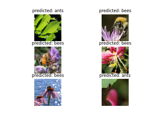
將卷積網路作為固定的特徵提取器#
在這裡,我們需要凍結除了最後一層之外的所有網路。我們需要將 requires_grad = False 來凍結引數,以便在 backward() 中不計算梯度。
您可以在文件 這裡 中閱讀更多關於此內容的資訊。
model_conv = torchvision.models.resnet18(weights='IMAGENET1K_V1')
for param in model_conv.parameters():
    param.requires_grad = False

# Parameters of newly constructed modules have requires_grad=True by default
num_ftrs = model_conv.fc.in_features
model_conv.fc = nn.Linear(num_ftrs, 2)

model_conv = model_conv.to(device)

criterion = nn.CrossEntropyLoss()

# Observe that only parameters of final layer are being optimized as
# opposed to before.
optimizer_conv = optim.SGD(model_conv.fc.parameters(), lr=0.001, momentum=0.9)

# Decay LR by a factor of 0.1 every 7 epochs
exp_lr_scheduler = lr_scheduler.StepLR(optimizer_conv, step_size=7, gamma=0.1)
訓練和評估#
在 CPU 上,這大約需要前一種情況一半的時間。這是預期的,因為大多數網路不需要計算梯度。但是,前向傳播仍然需要計算。
model_conv = train_model(model_conv, criterion, optimizer_conv,
                         exp_lr_scheduler, num_epochs=25)
Epoch 0/24
----------
train Loss: 0.6005 Acc: 0.6516
val Loss: 0.3484 Acc: 0.8497

Epoch 1/24
----------
train Loss: 0.4055 Acc: 0.8074
val Loss: 0.1546 Acc: 0.9477

Epoch 2/24
----------
train Loss: 0.3788 Acc: 0.8238
val Loss: 0.2740 Acc: 0.8889

Epoch 3/24
----------
train Loss: 0.4735 Acc: 0.8074
val Loss: 0.1895 Acc: 0.9346

Epoch 4/24
----------
train Loss: 0.4034 Acc: 0.8402
val Loss: 0.1625 Acc: 0.9346

Epoch 5/24
----------
train Loss: 0.3522 Acc: 0.8443
val Loss: 0.1662 Acc: 0.9542

Epoch 6/24
----------
train Loss: 0.5148 Acc: 0.7664
val Loss: 0.5580 Acc: 0.7974

Epoch 7/24
----------
train Loss: 0.5086 Acc: 0.7910
val Loss: 0.1755 Acc: 0.9542

Epoch 8/24
----------
train Loss: 0.3373 Acc: 0.8279
val Loss: 0.2159 Acc: 0.9412

Epoch 9/24
----------
train Loss: 0.3281 Acc: 0.8525
val Loss: 0.1755 Acc: 0.9477

Epoch 10/24
----------
train Loss: 0.3662 Acc: 0.8648
val Loss: 0.1813 Acc: 0.9542

Epoch 11/24
----------
train Loss: 0.3764 Acc: 0.8279
val Loss: 0.1766 Acc: 0.9477

Epoch 12/24
----------
train Loss: 0.3467 Acc: 0.8361
val Loss: 0.2039 Acc: 0.9412

Epoch 13/24
----------
train Loss: 0.2729 Acc: 0.8730
val Loss: 0.1693 Acc: 0.9542

Epoch 14/24
----------
train Loss: 0.4085 Acc: 0.8156
val Loss: 0.1752 Acc: 0.9542

Epoch 15/24
----------
train Loss: 0.3271 Acc: 0.8852
val Loss: 0.1763 Acc: 0.9542

Epoch 16/24
----------
train Loss: 0.3405 Acc: 0.8402
val Loss: 0.1858 Acc: 0.9608

Epoch 17/24
----------
train Loss: 0.2761 Acc: 0.9016
val Loss: 0.1821 Acc: 0.9542

Epoch 18/24
----------
train Loss: 0.3294 Acc: 0.8320
val Loss: 0.2104 Acc: 0.9412

Epoch 19/24
----------
train Loss: 0.2609 Acc: 0.8893
val Loss: 0.1764 Acc: 0.9542

Epoch 20/24
----------
train Loss: 0.3810 Acc: 0.8443
val Loss: 0.1840 Acc: 0.9477

Epoch 21/24
----------
train Loss: 0.3185 Acc: 0.8525
val Loss: 0.1795 Acc: 0.9477

Epoch 22/24
----------
train Loss: 0.3281 Acc: 0.8811
val Loss: 0.2054 Acc: 0.9412

Epoch 23/24
----------
train Loss: 0.3509 Acc: 0.8443
val Loss: 0.2059 Acc: 0.9412

Epoch 24/24
----------
train Loss: 0.3028 Acc: 0.8443
val Loss: 0.1932 Acc: 0.9542

Training complete in 0m 28s
Best val Acc: 0.960784
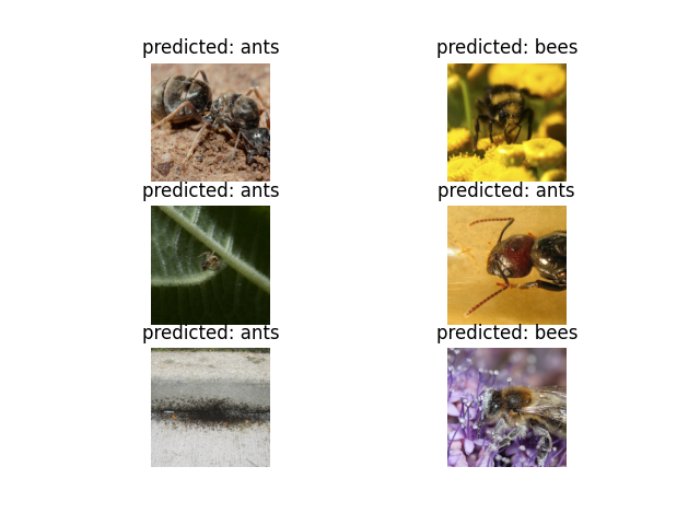
visualize_model(model_conv)

plt.ioff()
plt.show()
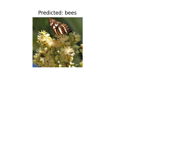
在自定義影像上進行推理#
使用訓練好的模型在自定義影像上進行預測,並可視化預測的類別標籤以及影像。
def visualize_model_predictions(model,img_path):
    was_training = model.training
    model.eval()

    img = Image.open(img_path)
    img = data_transforms['val'](img)
    img = img.unsqueeze(0)
    img = img.to(device)

    with torch.no_grad():
        outputs = model(img)
        _, preds = torch.max(outputs, 1)

        ax = plt.subplot(2,2,1)
        ax.axis('off')
        ax.set_title(f'Predicted: {class_names[preds[0]]}')
        imshow(img.cpu().data[0])

        model.train(mode=was_training)
visualize_model_predictions(
    model_conv,
    img_path='data/hymenoptera_data/val/bees/72100438_73de9f17af.jpg'
)

plt.ioff()
plt.show()
進一步學習#
如果您想了解更多關於遷移學習的應用,請檢視我們的 計算機視覺量化遷移學習教程。
指令碼總執行時間: (1 分鐘 6.486 秒)
