intermediate/spatial_transformer_tutorial

在 Google Colab 中執行
Colab

下載 Notebook
Notebook

在 GitHub 上檢視
GitHub
注意
轉到末尾 下載完整的示例程式碼。
空間變換網路教程#
創建於:2017年11月08日 | 最後更新:2024年01月19日 | 最後驗證:2024年11月05日
作者: Ghassen HAMROUNI
在本教程中,您將學習如何使用一種稱為空間變換網路的視覺注意力機制來增強您的網路。您可以閱讀更多關於空間變換網路的資訊,請參閱 DeepMind 論文
空間變換網路是對任何空間變換的可微分注意力的泛化。空間變換網路(簡稱 STN)允許神經網路學習如何對輸入影像執行空間變換,以增強模型的幾何不變性。例如,它可以裁剪感興趣的區域,縮放和校正影像的方向。這可能是一個有用的機制,因為卷積神經網路(CNN)對旋轉、縮放以及更一般的仿射變換不是不變的。
STN 的一個優點是,只需進行很少的修改就可以將其插入任何現有的 CNN 中。
# License: BSD
# Author: Ghassen Hamrouni

import torch
import torch.nn as nn
import torch.nn.functional as F
import torch.optim as optim
import torchvision
from torchvision import datasets, transforms
import matplotlib.pyplot as plt
import numpy as np

plt.ion()   # interactive mode
<contextlib.ExitStack object at 0x7f2cfd4906d0>
載入資料#
在這篇文章中,我們嘗試使用經典的 MNIST 資料集。使用帶有空間變換網路的標準卷積網路。
from six.moves import urllib
opener = urllib.request.build_opener()
opener.addheaders = [('User-agent', 'Mozilla/5.0')]
urllib.request.install_opener(opener)

device = torch.device("cuda" if torch.cuda.is_available() else "cpu")

# Training dataset
train_loader = torch.utils.data.DataLoader(
    datasets.MNIST(root='.', train=True, download=True,
                   transform=transforms.Compose([
                       transforms.ToTensor(),
                       transforms.Normalize((0.1307,), (0.3081,))
                   ])), batch_size=64, shuffle=True, num_workers=4)
# Test dataset
test_loader = torch.utils.data.DataLoader(
    datasets.MNIST(root='.', train=False, transform=transforms.Compose([
        transforms.ToTensor(),
        transforms.Normalize((0.1307,), (0.3081,))
    ])), batch_size=64, shuffle=True, num_workers=4)
  0%|          | 0.00/9.91M [00:00<?, ?B/s]
100%|██████████| 9.91M/9.91M [00:00<00:00, 148MB/s]

  0%|          | 0.00/28.9k [00:00<?, ?B/s]
100%|██████████| 28.9k/28.9k [00:00<00:00, 21.2MB/s]

  0%|          | 0.00/1.65M [00:00<?, ?B/s]
100%|██████████| 1.65M/1.65M [00:00<00:00, 293MB/s]

  0%|          | 0.00/4.54k [00:00<?, ?B/s]
100%|██████████| 4.54k/4.54k [00:00<00:00, 28.0MB/s]
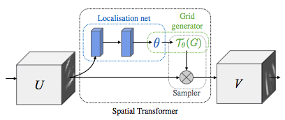
描繪空間變換網路#
空間變換網路歸結為三個主要組成部分:
定位網路是一個常規的 CNN,用於迴歸變換引數。變換不是從資料集中顯式學習的,而是網路自動學習增強全域性準確性的空間變換。
網格生成器在輸入影像中為輸出影像的每個畫素生成一個座標網格。
取樣器使用變換的引數並將其應用於輸入影像。
注意
我們需要最新版本的 PyTorch,其中包含 affine_grid 和 grid_sample 模組。
class Net(nn.Module):
    def __init__(self):
        super(Net, self).__init__()
        self.conv1 = nn.Conv2d(1, 10, kernel_size=5)
        self.conv2 = nn.Conv2d(10, 20, kernel_size=5)
        self.conv2_drop = nn.Dropout2d()
        self.fc1 = nn.Linear(320, 50)
        self.fc2 = nn.Linear(50, 10)

        # Spatial transformer localization-network
        self.localization = nn.Sequential(
            nn.Conv2d(1, 8, kernel_size=7),
            nn.MaxPool2d(2, stride=2),
            nn.ReLU(True),
            nn.Conv2d(8, 10, kernel_size=5),
            nn.MaxPool2d(2, stride=2),
            nn.ReLU(True)
        )

        # Regressor for the 3 * 2 affine matrix
        self.fc_loc = nn.Sequential(
            nn.Linear(10 * 3 * 3, 32),
            nn.ReLU(True),
            nn.Linear(32, 3 * 2)
        )

        # Initialize the weights/bias with identity transformation
        self.fc_loc[2].weight.data.zero_()
        self.fc_loc[2].bias.data.copy_(torch.tensor([1, 0, 0, 0, 1, 0], dtype=torch.float))

    # Spatial transformer network forward function
    def stn(self, x):
        xs = self.localization(x)
        xs = xs.view(-1, 10 * 3 * 3)
        theta = self.fc_loc(xs)
        theta = theta.view(-1, 2, 3)

        grid = F.affine_grid(theta, x.size())
        x = F.grid_sample(x, grid)

        return x

    def forward(self, x):
        # transform the input
        x = self.stn(x)

        # Perform the usual forward pass
        x = F.relu(F.max_pool2d(self.conv1(x), 2))
        x = F.relu(F.max_pool2d(self.conv2_drop(self.conv2(x)), 2))
        x = x.view(-1, 320)
        x = F.relu(self.fc1(x))
        x = F.dropout(x, training=self.training)
        x = self.fc2(x)
        return F.log_softmax(x, dim=1)


model = Net().to(device)
訓練模型#
現在,我們將使用 SGD 演算法來訓練模型。網路以監督方式學習分類任務。同時,模型以端到端的方式自動學習 STN。
optimizer = optim.SGD(model.parameters(), lr=0.01)


def train(epoch):
    model.train()
    for batch_idx, (data, target) in enumerate(train_loader):
        data, target = data.to(device), target.to(device)

        optimizer.zero_grad()
        output = model(data)
        loss = F.nll_loss(output, target)
        loss.backward()
        optimizer.step()
        if batch_idx % 500 == 0:
            print('Train Epoch: {} [{}/{} ({:.0f}%)]\tLoss: {:.6f}'.format(
                epoch, batch_idx * len(data), len(train_loader.dataset),
                100. * batch_idx / len(train_loader), loss.item()))
#
# A simple test procedure to measure the STN performances on MNIST.
#


def test():
    with torch.no_grad():
        model.eval()
        test_loss = 0
        correct = 0
        for data, target in test_loader:
            data, target = data.to(device), target.to(device)
            output = model(data)

            # sum up batch loss
            test_loss += F.nll_loss(output, target, size_average=False).item()
            # get the index of the max log-probability
            pred = output.max(1, keepdim=True)[1]
            correct += pred.eq(target.view_as(pred)).sum().item()

        test_loss /= len(test_loader.dataset)
        print('\nTest set: Average loss: {:.4f}, Accuracy: {}/{} ({:.0f}%)\n'
              .format(test_loss, correct, len(test_loader.dataset),
                      100. * correct / len(test_loader.dataset)))
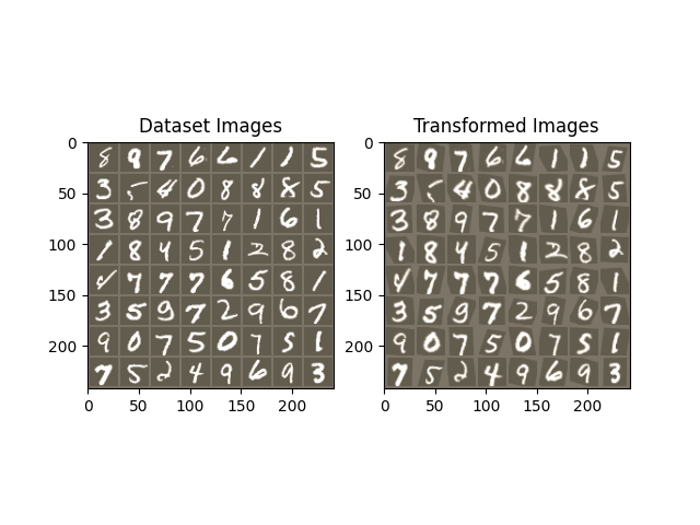
視覺化 STN 結果#
現在,我們將檢查我們學習到的視覺注意力機制的結果。
我們定義了一個小型輔助函式來視覺化訓練過程中的變換。
def convert_image_np(inp):
    """Convert a Tensor to numpy image."""
    inp = inp.numpy().transpose((1, 2, 0))
    mean = np.array([0.485, 0.456, 0.406])
    std = np.array([0.229, 0.224, 0.225])
    inp = std * inp + mean
    inp = np.clip(inp, 0, 1)
    return inp

# We want to visualize the output of the spatial transformers layer
# after the training, we visualize a batch of input images and
# the corresponding transformed batch using STN.


def visualize_stn():
    with torch.no_grad():
        # Get a batch of training data
        data = next(iter(test_loader))[0].to(device)

        input_tensor = data.cpu()
        transformed_input_tensor = model.stn(data).cpu()

        in_grid = convert_image_np(
            torchvision.utils.make_grid(input_tensor))

        out_grid = convert_image_np(
            torchvision.utils.make_grid(transformed_input_tensor))

        # Plot the results side-by-side
        f, axarr = plt.subplots(1, 2)
        axarr[0].imshow(in_grid)
        axarr[0].set_title('Dataset Images')

        axarr[1].imshow(out_grid)
        axarr[1].set_title('Transformed Images')

for epoch in range(1, 20 + 1):
    train(epoch)
    test()

# Visualize the STN transformation on some input batch
visualize_stn()

plt.ioff()
plt.show()
/usr/local/lib/python3.10/dist-packages/torch/nn/functional.py:5167: UserWarning:

Default grid_sample and affine_grid behavior has changed to align_corners=False since 1.3.0. Please specify align_corners=True if the old behavior is desired. See the documentation of grid_sample for details.

/usr/local/lib/python3.10/dist-packages/torch/nn/functional.py:5100: UserWarning:

Default grid_sample and affine_grid behavior has changed to align_corners=False since 1.3.0. Please specify align_corners=True if the old behavior is desired. See the documentation of grid_sample for details.

Train Epoch: 1 [0/60000 (0%)]   Loss: 2.321845
Train Epoch: 1 [32000/60000 (53%)]      Loss: 0.739860
/usr/local/lib/python3.10/dist-packages/torch/nn/_reduction.py:51: UserWarning:

size_average and reduce args will be deprecated, please use reduction='sum' instead.


Test set: Average loss: 0.2149, Accuracy: 9381/10000 (94%)

Train Epoch: 2 [0/60000 (0%)]   Loss: 0.310411
Train Epoch: 2 [32000/60000 (53%)]      Loss: 0.443614

Test set: Average loss: 0.1403, Accuracy: 9581/10000 (96%)

Train Epoch: 3 [0/60000 (0%)]   Loss: 0.184066
Train Epoch: 3 [32000/60000 (53%)]      Loss: 0.237139

Test set: Average loss: 0.0851, Accuracy: 9721/10000 (97%)

Train Epoch: 4 [0/60000 (0%)]   Loss: 0.235744
Train Epoch: 4 [32000/60000 (53%)]      Loss: 0.374082

Test set: Average loss: 0.0717, Accuracy: 9783/10000 (98%)

Train Epoch: 5 [0/60000 (0%)]   Loss: 0.209939
Train Epoch: 5 [32000/60000 (53%)]      Loss: 0.106230

Test set: Average loss: 0.0677, Accuracy: 9797/10000 (98%)

Train Epoch: 6 [0/60000 (0%)]   Loss: 0.210056
Train Epoch: 6 [32000/60000 (53%)]      Loss: 0.252697

Test set: Average loss: 0.0668, Accuracy: 9783/10000 (98%)

Train Epoch: 7 [0/60000 (0%)]   Loss: 0.123260
Train Epoch: 7 [32000/60000 (53%)]      Loss: 0.127563

Test set: Average loss: 0.0553, Accuracy: 9835/10000 (98%)

Train Epoch: 8 [0/60000 (0%)]   Loss: 0.108394
Train Epoch: 8 [32000/60000 (53%)]      Loss: 0.029457

Test set: Average loss: 0.0483, Accuracy: 9840/10000 (98%)

Train Epoch: 9 [0/60000 (0%)]   Loss: 0.176748
Train Epoch: 9 [32000/60000 (53%)]      Loss: 0.127248

Test set: Average loss: 0.1173, Accuracy: 9636/10000 (96%)

Train Epoch: 10 [0/60000 (0%)]  Loss: 0.243940
Train Epoch: 10 [32000/60000 (53%)]     Loss: 0.156468

Test set: Average loss: 0.2388, Accuracy: 9345/10000 (93%)

Train Epoch: 11 [0/60000 (0%)]  Loss: 0.378354
Train Epoch: 11 [32000/60000 (53%)]     Loss: 0.059640

Test set: Average loss: 0.0448, Accuracy: 9862/10000 (99%)

Train Epoch: 12 [0/60000 (0%)]  Loss: 0.129616
Train Epoch: 12 [32000/60000 (53%)]     Loss: 0.052506

Test set: Average loss: 0.0436, Accuracy: 9868/10000 (99%)

Train Epoch: 13 [0/60000 (0%)]  Loss: 0.045932
Train Epoch: 13 [32000/60000 (53%)]     Loss: 0.079384

Test set: Average loss: 0.0446, Accuracy: 9858/10000 (99%)

Train Epoch: 14 [0/60000 (0%)]  Loss: 0.031097
Train Epoch: 14 [32000/60000 (53%)]     Loss: 0.106284

Test set: Average loss: 0.0422, Accuracy: 9874/10000 (99%)

Train Epoch: 15 [0/60000 (0%)]  Loss: 0.133345
Train Epoch: 15 [32000/60000 (53%)]     Loss: 0.106248

Test set: Average loss: 0.0414, Accuracy: 9873/10000 (99%)

Train Epoch: 16 [0/60000 (0%)]  Loss: 0.044279
Train Epoch: 16 [32000/60000 (53%)]     Loss: 0.046603

Test set: Average loss: 0.0626, Accuracy: 9806/10000 (98%)

Train Epoch: 17 [0/60000 (0%)]  Loss: 0.157027
Train Epoch: 17 [32000/60000 (53%)]     Loss: 0.127502

Test set: Average loss: 0.0497, Accuracy: 9851/10000 (99%)

Train Epoch: 18 [0/60000 (0%)]  Loss: 0.041967
Train Epoch: 18 [32000/60000 (53%)]     Loss: 0.137598

Test set: Average loss: 0.0397, Accuracy: 9887/10000 (99%)

Train Epoch: 19 [0/60000 (0%)]  Loss: 0.115559
Train Epoch: 19 [32000/60000 (53%)]     Loss: 0.034766

Test set: Average loss: 0.0362, Accuracy: 9894/10000 (99%)

Train Epoch: 20 [0/60000 (0%)]  Loss: 0.078510
Train Epoch: 20 [32000/60000 (53%)]     Loss: 0.096980

Test set: Average loss: 0.0715, Accuracy: 9794/10000 (98%)
指令碼總執行時間: (1 分鐘 36.699 秒)
