視覺化工具

注意

在 Colab 中嘗試，或 轉到末尾 下載完整的示例程式碼。

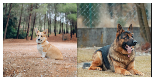
本示例展示了 torchvision 為視覺化影像、邊界框、分割掩碼和關鍵點提供的一些實用工具。

import torch
import numpy as np
import matplotlib.pyplot as plt

import torchvision.transforms.functional as F


plt.rcParams["savefig.bbox"] = 'tight'


def show(imgs):
    if not isinstance(imgs, list):
        imgs = [imgs]
    fig, axs = plt.subplots(ncols=len(imgs), squeeze=False)
    for i, img in enumerate(imgs):
        img = img.detach()
        img = F.to_pil_image(img)
        axs[0, i].imshow(np.asarray(img))
        axs[0, i].set(xticklabels=[], yticklabels=[], xticks=[], yticks=[])

視覺化影像網格

make_grid() 函式可用於建立一個表示網格中多張影像的張量。此實用程式需要 uint8 型別的單張影像作為輸入。

from torchvision.utils import make_grid
from torchvision.io import decode_image
from pathlib import Path

dog1_int = decode_image(str(Path('../assets') / 'dog1.jpg'))
dog2_int = decode_image(str(Path('../assets') / 'dog2.jpg'))
dog_list = [dog1_int, dog2_int]

grid = make_grid(dog_list)
show(grid)

視覺化邊界框

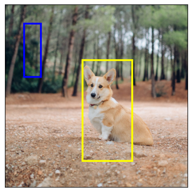
我們可以使用 draw_bounding_boxes() 在影像上繪製框。我們可以設定顏色、標籤、寬度以及字型和字型大小。框的格式為 (xmin, ymin, xmax, ymax)。

from torchvision.utils import draw_bounding_boxes


boxes = torch.tensor([[50, 50, 100, 200], [210, 150, 350, 430]], dtype=torch.float)
colors = ["blue", "yellow"]
result = draw_bounding_boxes(dog1_int, boxes, colors=colors, width=5)
show(result)

自然地，我們也可以繪製 torchvision 檢測模型產生的邊界框。這裡有一個使用從 fasterrcnn_resnet50_fpn() 模型載入的 Faster R-CNN 模型的演示。有關此類模型輸出的更多詳細資訊，請參閱 例項分割模型。

from torchvision.models.detection import fasterrcnn_resnet50_fpn, FasterRCNN_ResNet50_FPN_Weights


weights = FasterRCNN_ResNet50_FPN_Weights.DEFAULT
transforms = weights.transforms()

images = [transforms(d) for d in dog_list]

model = fasterrcnn_resnet50_fpn(weights=weights, progress=False)
model = model.eval()

outputs = model(images)
print(outputs)

[{'boxes': tensor([[215.9767, 171.1661, 402.0078, 378.7391],
        [344.6341, 172.6735, 357.6114, 220.1435],
        [153.1306, 185.5567, 172.9223, 254.7014]], grad_fn=<StackBackward0>), 'labels': tensor([18,  1,  1]), 'scores': tensor([0.9989, 0.0701, 0.0611], grad_fn=<IndexBackward0>)}, {'boxes': tensor([[ 23.5964, 132.4331, 449.9359, 493.0222],
        [225.8182, 124.6292, 467.2861, 492.2621],
        [ 18.5248, 135.4171, 420.9786, 479.2225]], grad_fn=<StackBackward0>), 'labels': tensor([18, 18, 17]), 'scores': tensor([0.9980, 0.0879, 0.0671], grad_fn=<IndexBackward0>)}]

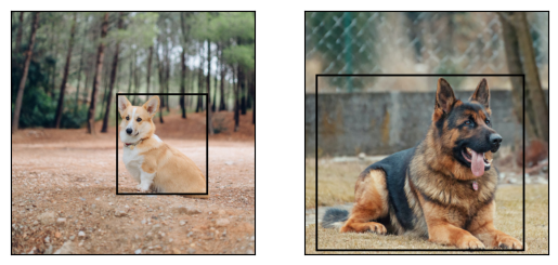
讓我們繪製模型檢測到的框。我們將只繪製分數大於給定閾值的框。

score_threshold = .8
dogs_with_boxes = [
    draw_bounding_boxes(dog_int, boxes=output['boxes'][output['scores'] > score_threshold], width=4)
    for dog_int, output in zip(dog_list, outputs)
]
show(dogs_with_boxes)

視覺化分割掩碼

draw_segmentation_masks() 函式可用於在影像上繪製分割掩碼。語義分割和例項分割模型的輸出不同，因此我們將分別處理它們。

語義分割模型

我們將瞭解如何使用 torchvision 的 FCN Resnet-50，透過 fcn_resnet50() 載入它。讓我們先看一下模型的輸出。

from torchvision.models.segmentation import fcn_resnet50, FCN_ResNet50_Weights

weights = FCN_ResNet50_Weights.DEFAULT
transforms = weights.transforms(resize_size=None)

model = fcn_resnet50(weights=weights, progress=False)
model = model.eval()

batch = torch.stack([transforms(d) for d in dog_list])
output = model(batch)['out']
print(output.shape, output.min().item(), output.max().item())

Downloading: "https://download.pytorch.org/models/fcn_resnet50_coco-1167a1af.pth" to /root/.cache/torch/hub/checkpoints/fcn_resnet50_coco-1167a1af.pth
torch.Size([2, 21, 500, 500]) -7.089669704437256 14.858257293701172

如上所示，分割模型的輸出是一個形狀為 (batch_size, num_classes, H, W) 的張量。每個值都是一個非歸一化的分數，我們可以透過使用 softmax 將它們歸一化到 [0, 1] 範圍。在 softmax 之後，我們可以將每個值解釋為機率，指示給定畫素屬於給定類的可能性。

讓我們繪製為狗類和船類檢測到的掩碼。

sem_class_to_idx = {cls: idx for (idx, cls) in enumerate(weights.meta["categories"])}

normalized_masks = torch.nn.functional.softmax(output, dim=1)

dog_and_boat_masks = [
    normalized_masks[img_idx, sem_class_to_idx[cls]]
    for img_idx in range(len(dog_list))
    for cls in ('dog', 'boat')
]

show(dog_and_boat_masks)

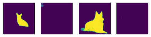
正如預期的那樣，模型對狗類非常有信心，但對船類信心不足。

draw_segmentation_masks() 函式可用於將這些掩碼繪製在原始影像之上。此函式需要布林掩碼，但我們上面的掩碼包含 [0, 1] 範圍內的機率。為了獲得布林掩碼，我們可以這樣做：

class_dim = 1
boolean_dog_masks = (normalized_masks.argmax(class_dim) == sem_class_to_idx['dog'])
print(f"shape = {boolean_dog_masks.shape}, dtype = {boolean_dog_masks.dtype}")
show([m.float() for m in boolean_dog_masks])

shape = torch.Size([2, 500, 500]), dtype = torch.bool

上面定義 boolean_dog_masks 的那一行有點晦澀，但您可以將其理解為以下查詢：“哪些畫素‘狗’是最有可能的類別？”

注意

雖然我們在這裡使用的是 normalized_masks，但如果我們直接使用模型的非歸一化分數，我們將得到相同的結果（因為 softmax 操作會保留順序）。

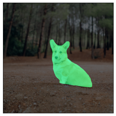
現在我們有了布林掩碼，我們可以使用 draw_segmentation_masks() 將它們繪製在原始影像之上。

from torchvision.utils import draw_segmentation_masks

dogs_with_masks = [
    draw_segmentation_masks(img, masks=mask, alpha=0.7)
    for img, mask in zip(dog_list, boolean_dog_masks)
]
show(dogs_with_masks)

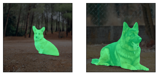
我們可以繪製多張影像的多個掩碼！請記住，模型返回的掩碼數量與類別的數量相同。讓我們問與上面相同的問題，但這次是針對所有類別，而不僅僅是狗類：“對於每個畫素和每個類別 C，類別 C 是最有可能的類別嗎？”

這個稍微複雜一些，所以我們將首先展示如何用單個影像完成，然後推廣到批處理。

num_classes = normalized_masks.shape[1]
dog1_masks = normalized_masks[0]
class_dim = 0
dog1_all_classes_masks = dog1_masks.argmax(class_dim) == torch.arange(num_classes)[:, None, None]

print(f"dog1_masks shape = {dog1_masks.shape}, dtype = {dog1_masks.dtype}")
print(f"dog1_all_classes_masks = {dog1_all_classes_masks.shape}, dtype = {dog1_all_classes_masks.dtype}")

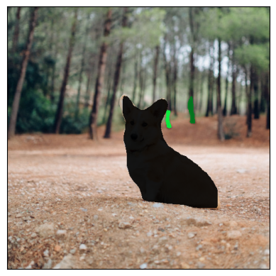
dog_with_all_masks = draw_segmentation_masks(dog1_int, masks=dog1_all_classes_masks, alpha=.6)
show(dog_with_all_masks)

dog1_masks shape = torch.Size([21, 500, 500]), dtype = torch.float32
dog1_all_classes_masks = torch.Size([21, 500, 500]), dtype = torch.bool

在上面的影像中，我們可以看到只繪製了兩個掩碼：背景掩碼和狗掩碼。這是因為模型認為只有這兩個類別是所有畫素中最有可能的。如果模型將另一個類別檢測為其他畫素中最有可能的類別，我們將在上面看到它的掩碼。

透過傳遞 masks=dog1_all_classes_masks[1:] 即可輕鬆移除背景掩碼，因為背景類別是索引為 0 的類別。

現在讓我們對整批影像做同樣的事情。程式碼類似，但涉及更多的維度處理。

class_dim = 1
all_classes_masks = normalized_masks.argmax(class_dim) == torch.arange(num_classes)[:, None, None, None]
print(f"shape = {all_classes_masks.shape}, dtype = {all_classes_masks.dtype}")
# The first dimension is the classes now, so we need to swap it
all_classes_masks = all_classes_masks.swapaxes(0, 1)

dogs_with_masks = [
    draw_segmentation_masks(img, masks=mask, alpha=.6)
    for img, mask in zip(dog_list, all_classes_masks)
]
show(dogs_with_masks)

shape = torch.Size([21, 2, 500, 500]), dtype = torch.bool

例項分割模型

例項分割模型的輸出與語義分割模型有顯著不同。在這裡，我們將瞭解如何繪製此類模型的掩碼。讓我們先分析 Mask-RCNN 模型的輸出。請注意，這些模型不需要對影像進行歸一化，因此我們不需要使用歸一化批次。

注意

這裡我們將描述 Mask-RCNN 模型的輸出。 目標檢測、例項分割和人物關鍵點檢測 中的模型具有相似的輸出格式，但其中一些可能包含額外的額外資訊，例如 keypointrcnn_resnet50_fpn() 的關鍵點，而其中一些可能沒有掩碼，例如 fasterrcnn_resnet50_fpn()。

from torchvision.models.detection import maskrcnn_resnet50_fpn, MaskRCNN_ResNet50_FPN_Weights

weights = MaskRCNN_ResNet50_FPN_Weights.DEFAULT
transforms = weights.transforms()

images = [transforms(d) for d in dog_list]

model = maskrcnn_resnet50_fpn(weights=weights, progress=False)
model = model.eval()

output = model(images)
print(output)

Downloading: "https://download.pytorch.org/models/maskrcnn_resnet50_fpn_coco-bf2d0c1e.pth" to /root/.cache/torch/hub/checkpoints/maskrcnn_resnet50_fpn_coco-bf2d0c1e.pth
[{'boxes': tensor([[219.7444, 168.1722, 400.7378, 384.0263],
        [343.9716, 171.2287, 358.3447, 222.6263],
        [301.0303, 192.6917, 313.8879, 232.3154]], grad_fn=<StackBackward0>), 'labels': tensor([18,  1,  1]), 'scores': tensor([0.9987, 0.7187, 0.6525], grad_fn=<IndexBackward0>), 'masks': tensor([[[[0., 0., 0.,  ..., 0., 0., 0.],
          [0., 0., 0.,  ..., 0., 0., 0.],
          [0., 0., 0.,  ..., 0., 0., 0.],
          ...,
          [0., 0., 0.,  ..., 0., 0., 0.],
          [0., 0., 0.,  ..., 0., 0., 0.],
          [0., 0., 0.,  ..., 0., 0., 0.]]],


        [[[0., 0., 0.,  ..., 0., 0., 0.],
          [0., 0., 0.,  ..., 0., 0., 0.],
          [0., 0., 0.,  ..., 0., 0., 0.],
          ...,
          [0., 0., 0.,  ..., 0., 0., 0.],
          [0., 0., 0.,  ..., 0., 0., 0.],
          [0., 0., 0.,  ..., 0., 0., 0.]]],


        [[[0., 0., 0.,  ..., 0., 0., 0.],
          [0., 0., 0.,  ..., 0., 0., 0.],
          [0., 0., 0.,  ..., 0., 0., 0.],
          ...,
          [0., 0., 0.,  ..., 0., 0., 0.],
          [0., 0., 0.,  ..., 0., 0., 0.],
          [0., 0., 0.,  ..., 0., 0., 0.]]]], grad_fn=<UnsqueezeBackward0>)}, {'boxes': tensor([[ 44.6767, 137.9018, 446.5324, 487.3429],
        [  0.0000, 288.0053, 489.9292, 490.2352]], grad_fn=<StackBackward0>), 'labels': tensor([18, 15]), 'scores': tensor([0.9978, 0.0697], grad_fn=<IndexBackward0>), 'masks': tensor([[[[0., 0., 0.,  ..., 0., 0., 0.],
          [0., 0., 0.,  ..., 0., 0., 0.],
          [0., 0., 0.,  ..., 0., 0., 0.],
          ...,
          [0., 0., 0.,  ..., 0., 0., 0.],
          [0., 0., 0.,  ..., 0., 0., 0.],
          [0., 0., 0.,  ..., 0., 0., 0.]]],


        [[[0., 0., 0.,  ..., 0., 0., 0.],
          [0., 0., 0.,  ..., 0., 0., 0.],
          [0., 0., 0.,  ..., 0., 0., 0.],
          ...,
          [0., 0., 0.,  ..., 0., 0., 0.],
          [0., 0., 0.,  ..., 0., 0., 0.],
          [0., 0., 0.,  ..., 0., 0., 0.]]]], grad_fn=<UnsqueezeBackward0>)}]

讓我們分解一下。對於批處理中的每張影像，模型都會輸出一些檢測（或例項）。每次影像的檢測數量不同。每個例項都由其邊界框、標籤、分數和掩碼描述。

輸出的組織方式如下：輸出是一個長度為 batch_size 的列表。列表中的每個條目對應一張輸入影像，它是一個包含 'boxes'、'labels'、'scores' 和 'masks' 鍵的字典。與這些鍵關聯的每個值都包含 num_instances 個元素。在上面的示例中，第一張影像檢測到 3 個例項，第二張影像檢測到 2 個例項。

可以使用 draw_bounding_boxes() 繪製框，但這裡我們更關注掩碼。這些掩碼與我們之前看到的用於語義分割模型的掩碼截然不同。

dog1_output = output[0]
dog1_masks = dog1_output['masks']
print(f"shape = {dog1_masks.shape}, dtype = {dog1_masks.dtype}, "
      f"min = {dog1_masks.min()}, max = {dog1_masks.max()}")

shape = torch.Size([3, 1, 500, 500]), dtype = torch.float32, min = 0.0, max = 0.9999862909317017

這裡的掩碼對應於機率，指示每個畫素屬於該例項的預測標籤的可能性。這些預測標籤對應於同一輸出字典中的 'labels' 元素。讓我們看看第一張影像例項的預測標籤。

print("For the first dog, the following instances were detected:")
print([weights.meta["categories"][label] for label in dog1_output['labels']])

For the first dog, the following instances were detected:
['dog', 'person', 'person']

有趣的是，模型檢測到了影像中的兩個人。讓我們繼續繪製這些掩碼。由於 draw_segmentation_masks() 需要布林掩碼，我們需要將這些機率轉換為布林值。請記住，這些掩碼的語義是“這個畫素屬於預測類的可能性有多大？”。因此，將這些掩碼轉換為布林值的一種自然方法是用 0.5 機率對其進行閾值處理（也可以選擇不同的閾值）。

proba_threshold = 0.5
dog1_bool_masks = dog1_output['masks'] > proba_threshold
print(f"shape = {dog1_bool_masks.shape}, dtype = {dog1_bool_masks.dtype}")

# There's an extra dimension (1) to the masks. We need to remove it
dog1_bool_masks = dog1_bool_masks.squeeze(1)

show(draw_segmentation_masks(dog1_int, dog1_bool_masks, alpha=0.9))

shape = torch.Size([3, 1, 500, 500]), dtype = torch.bool

模型似乎正確地檢測到了狗，但也將其誤認為人。仔細檢視分數將有助於我們繪製更有意義的掩碼。

print(dog1_output['scores'])

tensor([0.9987, 0.7187, 0.6525], grad_fn=<IndexBackward0>)

顯然，模型對狗的檢測比對人的檢測更有信心。這是個好訊息。在繪製掩碼時，我們可以要求僅繪製得分較高的掩碼。這裡我們使用 0.75 的分數閾值，並繪製第二隻狗的掩碼。

score_threshold = .75

boolean_masks = [
    out['masks'][out['scores'] > score_threshold] > proba_threshold
    for out in output
]

dogs_with_masks = [
    draw_segmentation_masks(img, mask.squeeze(1))
    for img, mask in zip(dog_list, boolean_masks)
]
show(dogs_with_masks)

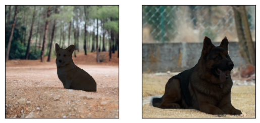
第一張影像中的兩個“人”掩碼未被選中，因為它們的得分低於分數閾值。同樣，在第二張影像中，類別為 15（對應於“長椅”）的例項未被選中。

視覺化關鍵點

draw_keypoints() 函式可用於在影像上繪製關鍵點。我們將瞭解如何使用 torchvision 的 KeypointRCNN，透過 keypointrcnn_resnet50_fpn() 載入它。我們首先看一下模型的輸出。

from torchvision.models.detection import keypointrcnn_resnet50_fpn, KeypointRCNN_ResNet50_FPN_Weights
from torchvision.io import decode_image

person_int = decode_image(str(Path("../assets") / "person1.jpg"))

weights = KeypointRCNN_ResNet50_FPN_Weights.DEFAULT
transforms = weights.transforms()

person_float = transforms(person_int)

model = keypointrcnn_resnet50_fpn(weights=weights, progress=False)
model = model.eval()

outputs = model([person_float])
print(outputs)

Downloading: "https://download.pytorch.org/models/keypointrcnn_resnet50_fpn_coco-fc266e95.pth" to /root/.cache/torch/hub/checkpoints/keypointrcnn_resnet50_fpn_coco-fc266e95.pth
[{'boxes': tensor([[124.3751, 177.9242, 327.6354, 574.7064],
        [124.3625, 180.7574, 290.1061, 390.7958]], grad_fn=<StackBackward0>), 'labels': tensor([1, 1]), 'scores': tensor([0.9998, 0.1070], grad_fn=<IndexBackward0>), 'keypoints': tensor([[[208.0176, 214.2408,   1.0000],
         [208.0176, 207.0375,   1.0000],
         [197.8246, 210.6392,   1.0000],
         [208.0176, 211.8398,   1.0000],
         [178.6378, 217.8425,   1.0000],
         [221.2086, 253.8590,   1.0000],
         [160.6502, 269.4662,   1.0000],
         [243.9929, 304.2822,   1.0000],
         [138.4655, 328.8935,   1.0000],
         [277.5698, 340.8990,   1.0000],
         [153.4551, 374.5144,   1.0000],
         [226.0053, 375.7150,   1.0000],
         [226.0053, 370.3125,   1.0000],
         [221.8082, 455.5516,   1.0000],
         [273.9723, 448.9486,   1.0000],
         [193.6275, 546.1932,   1.0000],
         [273.3727, 545.5930,   1.0000]],

        [[207.8327, 214.6636,   1.0000],
         [207.2343, 207.4622,   1.0000],
         [198.2590, 209.8627,   1.0000],
         [208.4310, 210.4628,   1.0000],
         [178.5134, 218.2642,   1.0000],
         [219.7997, 251.8704,   1.0000],
         [162.3579, 269.2736,   1.0000],
         [245.5288, 304.6800,   1.0000],
         [138.4238, 330.4848,   1.0000],
         [278.4382, 346.0876,   1.0000],
         [153.3826, 374.8929,   1.0000],
         [233.5618, 368.2917,   1.0000],
         [225.7832, 367.6916,   1.0000],
         [289.8069, 357.4897,   1.0000],
         [245.5288, 389.8956,   1.0000],
         [281.4300, 349.0882,   1.0000],
         [209.0294, 389.8956,   1.0000]]], grad_fn=<CopySlices>), 'keypoints_scores': tensor([[16.0164, 16.6672, 15.8312,  4.6510, 14.2053,  8.8280,  9.1136, 12.2084,
         12.1901, 13.8453, 10.7090,  5.5852,  7.5005, 11.3378,  9.3700,  8.2987,
          8.4479],
        [12.9326, 13.8158, 14.9053,  3.9368, 12.9585,  6.4240,  6.8328, 10.4227,
          9.2907, 10.1066, 10.1019,  0.1822,  4.3057, -4.9904, -2.7409, -2.7874,
         -3.9329]], grad_fn=<CopySlices>)}]

如我們所見，輸出包含一個字典列表。輸出列表的長度為 batch_size。我們目前只有一張影像，所以列表的長度為 1。列表中的每個條目對應一張輸入影像，它是一個包含 'boxes'、'labels'、'scores'、'keypoints' 和 'keypoint_scores' 鍵的字典。與這些鍵關聯的每個值都包含 num_instances 個元素。在上面的示例中，影像中檢測到 2 個例項。

kpts = outputs[0]['keypoints']
scores = outputs[0]['scores']

print(kpts)
print(scores)

tensor([[[208.0176, 214.2408,   1.0000],
         [208.0176, 207.0375,   1.0000],
         [197.8246, 210.6392,   1.0000],
         [208.0176, 211.8398,   1.0000],
         [178.6378, 217.8425,   1.0000],
         [221.2086, 253.8590,   1.0000],
         [160.6502, 269.4662,   1.0000],
         [243.9929, 304.2822,   1.0000],
         [138.4655, 328.8935,   1.0000],
         [277.5698, 340.8990,   1.0000],
         [153.4551, 374.5144,   1.0000],
         [226.0053, 375.7150,   1.0000],
         [226.0053, 370.3125,   1.0000],
         [221.8082, 455.5516,   1.0000],
         [273.9723, 448.9486,   1.0000],
         [193.6275, 546.1932,   1.0000],
         [273.3727, 545.5930,   1.0000]],

        [[207.8327, 214.6636,   1.0000],
         [207.2343, 207.4622,   1.0000],
         [198.2590, 209.8627,   1.0000],
         [208.4310, 210.4628,   1.0000],
         [178.5134, 218.2642,   1.0000],
         [219.7997, 251.8704,   1.0000],
         [162.3579, 269.2736,   1.0000],
         [245.5288, 304.6800,   1.0000],
         [138.4238, 330.4848,   1.0000],
         [278.4382, 346.0876,   1.0000],
         [153.3826, 374.8929,   1.0000],
         [233.5618, 368.2917,   1.0000],
         [225.7832, 367.6916,   1.0000],
         [289.8069, 357.4897,   1.0000],
         [245.5288, 389.8956,   1.0000],
         [281.4300, 349.0882,   1.0000],
         [209.0294, 389.8956,   1.0000]]], grad_fn=<CopySlices>)
tensor([0.9998, 0.1070], grad_fn=<IndexBackward0>)

KeypointRCNN 模型檢測到影像中有兩個例項。如果使用 draw_bounding_boxes() 繪製框，您會認出它們是人和衝浪板。如果我們檢視分數，會發現模型對人的信心遠高於對沖浪板。我們現在可以設定一個置信度閾值並繪製我們足夠自信的例項。讓我們將閾值設定為 0.75，並過濾出對應於人的關鍵點。

detect_threshold = 0.75
idx = torch.where(scores > detect_threshold)
keypoints = kpts[idx]

print(keypoints)

tensor([[[208.0176, 214.2408,   1.0000],
         [208.0176, 207.0375,   1.0000],
         [197.8246, 210.6392,   1.0000],
         [208.0176, 211.8398,   1.0000],
         [178.6378, 217.8425,   1.0000],
         [221.2086, 253.8590,   1.0000],
         [160.6502, 269.4662,   1.0000],
         [243.9929, 304.2822,   1.0000],
         [138.4655, 328.8935,   1.0000],
         [277.5698, 340.8990,   1.0000],
         [153.4551, 374.5144,   1.0000],
         [226.0053, 375.7150,   1.0000],
         [226.0053, 370.3125,   1.0000],
         [221.8082, 455.5516,   1.0000],
         [273.9723, 448.9486,   1.0000],
         [193.6275, 546.1932,   1.0000],
         [273.3727, 545.5930,   1.0000]]], grad_fn=<IndexBackward0>)

太好了，現在我們有了對應於人的關鍵點。每個關鍵點都由 x、y 座標和可見性表示。我們現在可以使用 draw_keypoints() 函式繪製關鍵點。請注意，該實用程式需要 uint8 影像。

from torchvision.utils import draw_keypoints

res = draw_keypoints(person_int, keypoints, colors="blue", radius=3)
show(res)

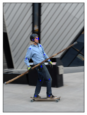
如我們所見，關鍵點顯示為影像上的彩色圓圈。人的 COCO 關鍵點是有序的，代表以下列表。

coco_keypoints = [
    "nose", "left_eye", "right_eye", "left_ear", "right_ear",
    "left_shoulder", "right_shoulder", "left_elbow", "right_elbow",
    "left_wrist", "right_wrist", "left_hip", "right_hip",
    "left_knee", "right_knee", "left_ankle", "right_ankle",
]

如果我們對連線關鍵點感興趣該怎麼辦？這在建立姿態檢測或動作識別時特別有用。我們可以使用 'connectivity' 引數輕鬆連線關鍵點。仔細觀察會發現，我們需要按以下順序連線點來構建人體骨骼。

鼻子 -> 左眼 -> 左耳。(0, 1), (1, 3)

鼻子 -> 右眼 -> 右耳。(0, 2), (2, 4)

鼻子 -> 左肩 -> 左肘 -> 左腕。(0, 5), (5, 7), (7, 9)

鼻子 -> 右肩 -> 右肘 -> 右腕。(0, 6), (6, 8), (8, 10)

左肩 -> 左髖 -> 左膝 -> 左踝。(5, 11), (11, 13), (13, 15)

右肩 -> 右髖 -> 右膝 -> 右踝。(6, 12), (12, 14), (14, 16)

我們將建立一個包含這些要連線的關鍵點 ID 的列表。

connect_skeleton = [
    (0, 1), (0, 2), (1, 3), (2, 4), (0, 5), (0, 6), (5, 7), (6, 8),
    (7, 9), (8, 10), (5, 11), (6, 12), (11, 13), (12, 14), (13, 15), (14, 16)
]

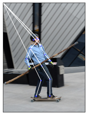
我們將上述列表傳遞給 connectivity 引數以連線關鍵點。

res = draw_keypoints(person_int, keypoints, connectivity=connect_skeleton, colors="blue", radius=4, width=3)
show(res)

看起來很不錯。

使用可見性繪製關鍵點

讓我們看看另一個關鍵點預測模組產生的結果，並顯示連線。

prediction = torch.tensor(
    [[[208.0176, 214.2409, 1.0000],
      [000.0000, 000.0000, 0.0000],
      [197.8246, 210.6392, 1.0000],
      [000.0000, 000.0000, 0.0000],
      [178.6378, 217.8425, 1.0000],
      [221.2086, 253.8591, 1.0000],
      [160.6502, 269.4662, 1.0000],
      [243.9929, 304.2822, 1.0000],
      [138.4654, 328.8935, 1.0000],
      [277.5698, 340.8990, 1.0000],
      [153.4551, 374.5145, 1.0000],
      [000.0000, 000.0000, 0.0000],
      [226.0053, 370.3125, 1.0000],
      [221.8081, 455.5516, 1.0000],
      [273.9723, 448.9486, 1.0000],
      [193.6275, 546.1933, 1.0000],
      [273.3727, 545.5930, 1.0000]]]
)

res = draw_keypoints(person_int, prediction, connectivity=connect_skeleton, colors="blue", radius=4, width=3)
show(res)

發生了什麼？預測新關鍵點的模型無法檢測到隱藏在滑板者上半身左側的三個點。更具體地說，模型預測左眼、左耳和左髖的 (x, y, vis) = (0, 0, 0)。因此，我們絕對不希望顯示這些關鍵點和連線，您也不必這樣做。檢視 draw_keypoints() 的引數，我們可以看到可以傳遞可見性張量作為附加引數。鑑於模型的預測，可見性是第三個關鍵點維度，我們只需要提取它。讓我們將 prediction 分割為關鍵點座標及其各自的可見性，並將兩者都作為引數傳遞給 draw_keypoints()。

coordinates, visibility = prediction.split([2, 1], dim=-1)
visibility = visibility.bool()

res = draw_keypoints(
    person_int, coordinates, visibility=visibility, connectivity=connect_skeleton, colors="blue", radius=4, width=3
)
show(res)

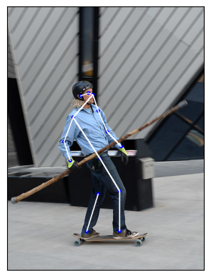
我們可以看到未檢測到的關鍵點未被繪製，並且不可見的連線被跳過。這可以減少多檢測影像或像我們這種情況（關鍵點預測模型遺漏了一些檢測）下的噪聲。大多數 torch 關鍵點預測模型會為每個預測返回可見性，供您使用。我們在第一個示例中使用的 keypointrcnn_resnet50_fpn() 模型也這樣做。