


注意
轉到底部 下載完整的示例程式碼。
從零開始的NLP:使用字元級RNN進行姓名分類#
建立時間:2017年3月24日 | 最後更新:2025年3月14日 | 最後驗證:2024年11月05日
作者: Sean Robertson
本教程是三部曲系列的一部分
我們將構建和訓練一個基本的字元級迴圈神經網路(RNN)來對單詞進行分類。本教程以及另外兩個自然語言處理(NLP)“從零開始”的教程 從零開始的NLP:使用字元級RNN生成姓名 和 從零開始的NLP:使用序列到序列網路和注意力機制進行翻譯,展示瞭如何預處理資料以模擬NLP。特別是,這些教程從底層展示了NLP資料的預處理是如何工作的。
字元級RNN將單詞讀取為一個字元序列——在每一步輸出一個預測和一個“隱藏狀態”,將其前一個隱藏狀態饋送到每一步。我們將最終預測作為輸出,即該單詞所屬的類別。
具體來說,我們將基於18種不同語言的數千個姓氏進行訓練,並根據拼寫預測一個姓名屬於哪種語言。
推薦準備#
在開始本教程之前,建議您已安裝PyTorch,並對Python程式語言和張量(Tensors)有基本瞭解。
https://pytorch.com.tw/ 獲取安裝說明
PyTorch深度學習:60分鐘速成班 以便全面瞭解PyTorch並學習張量的基礎知識。
透過例項學習PyTorch,進行廣泛而深入的概覽
為前Torch使用者準備的PyTorch教程,如果您是前Lua Torch使用者
瞭解RNN及其工作原理也會有所幫助。
迴圈神經網路的不可思議的有效性 展示了大量現實生活中的例子。
理解LSTM網路 主要講解LSTM,但也涵蓋了RNN的一般資訊。
準備Torch#
設定torch以預設使用正確的裝置,根據您的硬體(CPU或CUDA)進行GPU加速。
import torch

# Check if CUDA is available
device = torch.device('cpu')
if torch.cuda.is_available():
    device = torch.device('cuda')

torch.set_default_device(device)
print(f"Using device = {torch.get_default_device()}")
Using device = cuda:0
準備資料#
從此處下載資料並解壓到當前目錄。
在data/names目錄中包含18個文字檔案,檔名格式為[Language].txt。每個檔案包含大量姓名,每行一個姓名,大部分是羅馬化(但我們仍需要從Unicode轉換為ASCII)。
第一步是定義和清理我們的資料。首先,我們需要將Unicode轉換為純ASCII,以限制RNN的輸入層。這透過將Unicode字串轉換為ASCII並僅允許一小組允許的字元來實現。
import string
import unicodedata

# We can use "_" to represent an out-of-vocabulary character, that is, any character we are not handling in our model
allowed_characters = string.ascii_letters + " .,;'" + "_"
n_letters = len(allowed_characters)

# Turn a Unicode string to plain ASCII, thanks to https://stackoverflow.com/a/518232/2809427
def unicodeToAscii(s):
    return ''.join(
        c for c in unicodedata.normalize('NFD', s)
        if unicodedata.category(c) != 'Mn'
        and c in allowed_characters
    )
以下是將Unicode字母姓名轉換為純ASCII的示例。這簡化了輸入層。
print (f"converting 'Ślusàrski' to {unicodeToAscii('Ślusàrski')}")
converting 'Ślusàrski' to Slusarski
將姓名轉換為張量#
既然我們已經組織好了所有姓名,我們就需要將它們轉換為張量才能使用。
為了表示一個字母,我們使用一個大小為<1 x n_letters>的“獨熱編碼向量”(one-hot vector)。獨熱編碼向量除了在當前字母索引處為1之外,其餘位置都為0,例如"b" = <0 1 0 0 0 ...>。
為了構成一個單詞,我們將一堆這樣的向量連線成一個二維矩陣<line_length x 1 x n_letters>。
多出的一個維度是因為PyTorch假定所有東西都在批次中——我們這裡只使用了批次大小為1。
# Find letter index from all_letters, e.g. "a" = 0
def letterToIndex(letter):
    # return our out-of-vocabulary character if we encounter a letter unknown to our model
    if letter not in allowed_characters:
        return allowed_characters.find("_")
    else:
        return allowed_characters.find(letter)

# Turn a line into a <line_length x 1 x n_letters>,
# or an array of one-hot letter vectors
def lineToTensor(line):
    tensor = torch.zeros(len(line), 1, n_letters)
    for li, letter in enumerate(line):
        tensor[li][0][letterToIndex(letter)] = 1
    return tensor
以下是如何為單個字元或多個字元字串使用lineToTensor()的示例。
print (f"The letter 'a' becomes {lineToTensor('a')}") #notice that the first position in the tensor = 1
print (f"The name 'Ahn' becomes {lineToTensor('Ahn')}") #notice 'A' sets the 27th index to 1
The letter 'a' becomes tensor([[[1., 0., 0., 0., 0., 0., 0., 0., 0., 0., 0., 0., 0., 0., 0., 0., 0.,
          0., 0., 0., 0., 0., 0., 0., 0., 0., 0., 0., 0., 0., 0., 0., 0., 0.,
          0., 0., 0., 0., 0., 0., 0., 0., 0., 0., 0., 0., 0., 0., 0., 0., 0.,
          0., 0., 0., 0., 0., 0., 0.]]], device='cuda:0')
The name 'Ahn' becomes tensor([[[0., 0., 0., 0., 0., 0., 0., 0., 0., 0., 0., 0., 0., 0., 0., 0., 0.,
          0., 0., 0., 0., 0., 0., 0., 0., 0., 1., 0., 0., 0., 0., 0., 0., 0.,
          0., 0., 0., 0., 0., 0., 0., 0., 0., 0., 0., 0., 0., 0., 0., 0., 0.,
          0., 0., 0., 0., 0., 0., 0.]],

        [[0., 0., 0., 0., 0., 0., 0., 1., 0., 0., 0., 0., 0., 0., 0., 0., 0.,
          0., 0., 0., 0., 0., 0., 0., 0., 0., 0., 0., 0., 0., 0., 0., 0., 0.,
          0., 0., 0., 0., 0., 0., 0., 0., 0., 0., 0., 0., 0., 0., 0., 0., 0.,
          0., 0., 0., 0., 0., 0., 0.]],

        [[0., 0., 0., 0., 0., 0., 0., 0., 0., 0., 0., 0., 0., 1., 0., 0., 0.,
          0., 0., 0., 0., 0., 0., 0., 0., 0., 0., 0., 0., 0., 0., 0., 0., 0.,
          0., 0., 0., 0., 0., 0., 0., 0., 0., 0., 0., 0., 0., 0., 0., 0., 0.,
          0., 0., 0., 0., 0., 0., 0.]]], device='cuda:0')
恭喜您,您已經為這項學習任務構建了基礎的張量物件!您可以在其他涉及文字的RNN任務中使用類似的方法。
接下來,我們需要將所有示例組合成一個數據集,以便我們可以訓練、測試和驗證我們的模型。為此,我們將使用Dataset和DataLoader類來儲存我們的資料集。每個Dataset需要實現三個函式:__init__、__len__和__getitem__。
from io import open
import glob
import os
import time

import torch
from torch.utils.data import Dataset

class NamesDataset(Dataset):

    def __init__(self, data_dir):
        self.data_dir = data_dir #for provenance of the dataset
        self.load_time = time.localtime #for provenance of the dataset
        labels_set = set() #set of all classes

        self.data = []
        self.data_tensors = []
        self.labels = []
        self.labels_tensors = []

        #read all the ``.txt`` files in the specified directory
        text_files = glob.glob(os.path.join(data_dir, '*.txt'))
        for filename in text_files:
            label = os.path.splitext(os.path.basename(filename))[0]
            labels_set.add(label)
            lines = open(filename, encoding='utf-8').read().strip().split('\n')
            for name in lines:
                self.data.append(name)
                self.data_tensors.append(lineToTensor(name))
                self.labels.append(label)

        #Cache the tensor representation of the labels
        self.labels_uniq = list(labels_set)
        for idx in range(len(self.labels)):
            temp_tensor = torch.tensor([self.labels_uniq.index(self.labels[idx])], dtype=torch.long)
            self.labels_tensors.append(temp_tensor)

    def __len__(self):
        return len(self.data)

    def __getitem__(self, idx):
        data_item = self.data[idx]
        data_label = self.labels[idx]
        data_tensor = self.data_tensors[idx]
        label_tensor = self.labels_tensors[idx]

        return label_tensor, data_tensor, data_label, data_item
在這裡,我們可以將示例資料載入到NamesDataset中。
alldata = NamesDataset("data/names")
print(f"loaded {len(alldata)} items of data")
print(f"example = {alldata[0]}")
loaded 20074 items of data
example = (tensor([12], device='cuda:0'), tensor([[[0., 0., 0., 0., 0., 0., 0., 0., 0., 0., 0., 0., 0., 0., 0., 0., 0.,
          0., 0., 0., 0., 0., 0., 0., 0., 0., 0., 0., 0., 0., 0., 0., 0., 0.,
          0., 0., 1., 0., 0., 0., 0., 0., 0., 0., 0., 0., 0., 0., 0., 0., 0.,
          0., 0., 0., 0., 0., 0., 0.]],

        [[0., 0., 0., 0., 0., 0., 0., 1., 0., 0., 0., 0., 0., 0., 0., 0., 0.,
          0., 0., 0., 0., 0., 0., 0., 0., 0., 0., 0., 0., 0., 0., 0., 0., 0.,
          0., 0., 0., 0., 0., 0., 0., 0., 0., 0., 0., 0., 0., 0., 0., 0., 0.,
          0., 0., 0., 0., 0., 0., 0.]],

        [[0., 0., 0., 0., 0., 0., 0., 0., 0., 0., 0., 0., 0., 0., 1., 0., 0.,
          0., 0., 0., 0., 0., 0., 0., 0., 0., 0., 0., 0., 0., 0., 0., 0., 0.,
          0., 0., 0., 0., 0., 0., 0., 0., 0., 0., 0., 0., 0., 0., 0., 0., 0.,
          0., 0., 0., 0., 0., 0., 0.]],

        [[0., 0., 0., 0., 0., 0., 0., 0., 0., 0., 0., 0., 0., 0., 0., 0., 0.,
          0., 0., 0., 1., 0., 0., 0., 0., 0., 0., 0., 0., 0., 0., 0., 0., 0.,
          0., 0., 0., 0., 0., 0., 0., 0., 0., 0., 0., 0., 0., 0., 0., 0., 0.,
          0., 0., 0., 0., 0., 0., 0.]],

        [[0., 0., 0., 0., 0., 0., 0., 0., 0., 0., 0., 0., 0., 0., 0., 0., 0.,
          1., 0., 0., 0., 0., 0., 0., 0., 0., 0., 0., 0., 0., 0., 0., 0., 0.,
          0., 0., 0., 0., 0., 0., 0., 0., 0., 0., 0., 0., 0., 0., 0., 0., 0.,
          0., 0., 0., 0., 0., 0., 0.]],

        [[0., 0., 0., 0., 0., 0., 0., 0., 0., 0., 0., 0., 0., 0., 0., 0., 0.,
          0., 0., 0., 0., 0., 0., 0., 1., 0., 0., 0., 0., 0., 0., 0., 0., 0.,
          0., 0., 0., 0., 0., 0., 0., 0., 0., 0., 0., 0., 0., 0., 0., 0., 0.,
          0., 0., 0., 0., 0., 0., 0.]]], device='cuda:0'), 'Arabic', 'Khoury')
- 使用資料集物件可以讓我們輕鬆地將資料分割成訓練集和測試集。這裡我們建立了一個80/20
分割,但
torch.utils.data提供了更多有用的工具。這裡我們指定了一個生成器,因為我們需要使用
與PyTorch預設設定相同的裝置。
train_set, test_set = torch.utils.data.random_split(alldata, [.85, .15], generator=torch.Generator(device=device).manual_seed(2024))

print(f"train examples = {len(train_set)}, validation examples = {len(test_set)}")
train examples = 17063, validation examples = 3011
現在我們擁有了一個基本資料集,其中包含**20074**個示例,每個示例都是一個標籤和姓名的配對。我們還將資料集分割成了訓練集和測試集,以便我們可以驗證我們構建的模型。
建立網路#
在自動微分(autograd)出現之前,在Torch中建立一個迴圈神經網路需要在多個時間步上克隆一個層的引數。這些層持有現在完全由圖本身處理的隱藏狀態和梯度。這意味著您可以非常“純粹”地實現一個RNN,就像普通的饋通網路一樣。
這個CharRNN類實現了一個具有三個元件的RNN。首先,我們使用nn.RNN實現。接下來,我們定義一個將RNN隱藏層對映到我們輸出的層。最後,我們應用一個softmax函式。與將每個層實現為nn.Linear相比,使用nn.RNN可以顯著提高效能,例如cuDNN加速的核心。它也簡化了forward()中的實現。
import torch.nn as nn
import torch.nn.functional as F

class CharRNN(nn.Module):
    def __init__(self, input_size, hidden_size, output_size):
        super(CharRNN, self).__init__()

        self.rnn = nn.RNN(input_size, hidden_size)
        self.h2o = nn.Linear(hidden_size, output_size)
        self.softmax = nn.LogSoftmax(dim=1)

    def forward(self, line_tensor):
        rnn_out, hidden = self.rnn(line_tensor)
        output = self.h2o(hidden[0])
        output = self.softmax(output)

        return output
然後,我們可以建立一個具有58個輸入節點、128個隱藏節點和18個輸出的RNN。
n_hidden = 128
rnn = CharRNN(n_letters, n_hidden, len(alldata.labels_uniq))
print(rnn)
CharRNN(
  (rnn): RNN(58, 128)
  (h2o): Linear(in_features=128, out_features=18, bias=True)
  (softmax): LogSoftmax(dim=1)
)
之後,我們可以將張量傳遞給RNN以獲得預測輸出。隨後,我們使用一個名為label_from_output的輔助函式來從類別中提取文字標籤。
def label_from_output(output, output_labels):
    top_n, top_i = output.topk(1)
    label_i = top_i[0].item()
    return output_labels[label_i], label_i

input = lineToTensor('Albert')
output = rnn(input) #this is equivalent to ``output = rnn.forward(input)``
print(output)
print(label_from_output(output, alldata.labels_uniq))
tensor([[-2.8962, -2.8510, -2.8362, -3.0261, -2.9197, -2.8341, -2.8506, -2.9229,
         -2.9940, -2.9538, -2.8334, -2.8647, -2.9086, -2.8056, -2.8497, -2.8957,
         -2.8448, -2.9723]], device='cuda:0', grad_fn=<LogSoftmaxBackward0>)
('Spanish', 13)
訓練#
訓練網路#
現在訓練這個網路只需要給它看大量示例,讓它進行猜測,並告訴它是否錯了。
我們透過定義一個train()函式來實現這一點,該函式使用小批次(minibatches)在給定資料集上訓練模型。RNN與其他網路類似地進行訓練;因此,為完整起見,我們在此包含一個批次訓練方法。該迴圈(for i in batch)在調整權重之前計算批次中每個專案的損失。此操作會重複進行,直到達到指定的訓練輪數(epochs)。
import random
import numpy as np

def train(rnn, training_data, n_epoch = 10, n_batch_size = 64, report_every = 50, learning_rate = 0.2, criterion = nn.NLLLoss()):
    """
    Learn on a batch of training_data for a specified number of iterations and reporting thresholds
    """
    # Keep track of losses for plotting
    current_loss = 0
    all_losses = []
    rnn.train()
    optimizer = torch.optim.SGD(rnn.parameters(), lr=learning_rate)

    start = time.time()
    print(f"training on data set with n = {len(training_data)}")

    for iter in range(1, n_epoch + 1):
        rnn.zero_grad() # clear the gradients

        # create some minibatches
        # we cannot use dataloaders because each of our names is a different length
        batches = list(range(len(training_data)))
        random.shuffle(batches)
        batches = np.array_split(batches, len(batches) //n_batch_size )

        for idx, batch in enumerate(batches):
            batch_loss = 0
            for i in batch: #for each example in this batch
                (label_tensor, text_tensor, label, text) = training_data[i]
                output = rnn.forward(text_tensor)
                loss = criterion(output, label_tensor)
                batch_loss += loss

            # optimize parameters
            batch_loss.backward()
            nn.utils.clip_grad_norm_(rnn.parameters(), 3)
            optimizer.step()
            optimizer.zero_grad()

            current_loss += batch_loss.item() / len(batch)

        all_losses.append(current_loss / len(batches) )
        if iter % report_every == 0:
            print(f"{iter} ({iter / n_epoch:.0%}): \t average batch loss = {all_losses[-1]}")
        current_loss = 0

    return all_losses
我們現在可以為資料集使用小批次訓練,訓練指定的輪數。為了加快構建速度,本示例中的訓練輪數已減少。您可以使用不同的引數獲得更好的結果。
start = time.time()
all_losses = train(rnn, train_set, n_epoch=27, learning_rate=0.15, report_every=5)
end = time.time()
print(f"training took {end-start}s")
training on data set with n = 17063
5 (19%):         average batch loss = 0.877891722006078
10 (37%):        average batch loss = 0.6838399407782949
15 (56%):        average batch loss = 0.5772297213089955
20 (74%):        average batch loss = 0.48974639862051866
25 (93%):        average batch loss = 0.4353903183734024
training took 345.4310917854309s
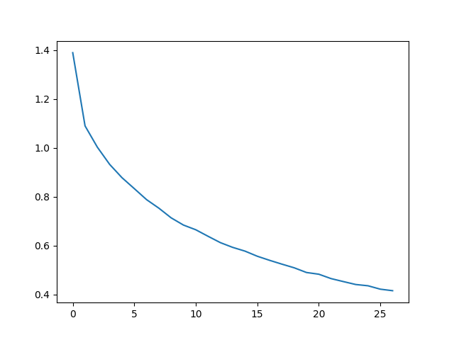
繪製結果#
繪製all_losses中的歷史損失圖,顯示網路正在學習。
import matplotlib.pyplot as plt
import matplotlib.ticker as ticker

plt.figure()
plt.plot(all_losses)
plt.show()
評估結果#
為了檢視網路在不同類別上的表現如何,我們將建立一個混淆矩陣,指示每個實際語言(行)的網路猜測的語言(列)。為了計算混淆矩陣,將一批樣本透過evaluate()函式傳遞給網路,這與train()函式相同,只是沒有反向傳播。
def evaluate(rnn, testing_data, classes):
    confusion = torch.zeros(len(classes), len(classes))

    rnn.eval() #set to eval mode
    with torch.no_grad(): # do not record the gradients during eval phase
        for i in range(len(testing_data)):
            (label_tensor, text_tensor, label, text) = testing_data[i]
            output = rnn(text_tensor)
            guess, guess_i = label_from_output(output, classes)
            label_i = classes.index(label)
            confusion[label_i][guess_i] += 1

    # Normalize by dividing every row by its sum
    for i in range(len(classes)):
        denom = confusion[i].sum()
        if denom > 0:
            confusion[i] = confusion[i] / denom

    # Set up plot
    fig = plt.figure()
    ax = fig.add_subplot(111)
    cax = ax.matshow(confusion.cpu().numpy()) #numpy uses cpu here so we need to use a cpu version
    fig.colorbar(cax)

    # Set up axes
    ax.set_xticks(np.arange(len(classes)), labels=classes, rotation=90)
    ax.set_yticks(np.arange(len(classes)), labels=classes)

    # Force label at every tick
    ax.xaxis.set_major_locator(ticker.MultipleLocator(1))
    ax.yaxis.set_major_locator(ticker.MultipleLocator(1))

    # sphinx_gallery_thumbnail_number = 2
    plt.show()


evaluate(rnn, test_set, classes=alldata.labels_uniq)
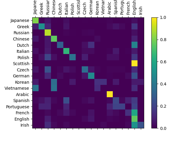
您可以從主對角線以外的亮點中看出它猜錯的語言,例如將韓語猜成中文,將義大利語猜成西班牙語。它似乎對希臘語表現得非常好,對英語表現得很差(可能是因為與其他語言有重疊)。
練習#
使用更大和/或形狀更好的網路可以獲得更好的結果。
調整超引數以提高效能,例如更改訓練輪數、批次大小和學習率。
嘗試使用
nn.LSTM和nn.GRU層。修改層的大小,例如增加或減少隱藏節點的數量,或新增額外的線性層。
將多個RNN組合成一個更高階的網路。
嘗試使用不同的行-標籤資料集,例如:
任何單詞 -> 語言
名字 -> 性別
字元名 -> 作者
頁面標題 -> 部落格或子版塊
指令碼總執行時間: (5 分鐘 51.591 秒)
