評價此頁

★ ★ ★ ★ ★

beginner/knowledge_distillation_tutorial

在 Google Colab 中執行

注意

轉到末尾下載完整的示例程式碼。

知識蒸餾教程#

建立日期：2023年8月22日 | 最後更新：2025年1月24日 | 最後驗證：2024年11月05日

作者： Alexandros Chariton

知識蒸餾是一種技術，它能夠將知識從大型、計算成本高昂的模型轉移到小型模型，同時不損失有效性。這使得模型可以在能力較弱的硬體上部署，從而使評估更快、更有效。

在本教程中，我們將進行一系列實驗，重點是提高輕量級神經網路的準確性，使用一個更強大的網路作為教師。輕量級網路的計算成本和速度將保持不變，我們的干預僅關注其權重，而不是其前向傳播。這項技術的應用可以在無人機或手機等裝置上找到。在本教程中，我們不使用任何外部包，因為我們需要的所有內容都可以在 torch 和 torchvision 中找到。

在本教程中，您將學到

如何修改模型類以提取隱藏表示並用於進一步計算
如何修改 PyTorch 中的常規訓練迴圈，在分類的交叉熵等損失之上新增額外的損失
如何透過使用更復雜的模型作為教師來提高輕量級模型的效能

先決條件#

1 塊 GPU，4GB 記憶體
PyTorch v2.0 或更高版本
CIFAR-10 資料集（由指令碼下載並儲存在名為 /data 的目錄中）

import torch
import torch.nn as nn
import torch.optim as optim
import torchvision.transforms as transforms
import torchvision.datasets as datasets

# Check if the current `accelerator <https://pytorch.com.tw/docs/stable/torch.html#accelerators>`__
# is available, and if not, use the CPU
device = torch.accelerator.current_accelerator().type if torch.accelerator.is_available() else "cpu"
print(f"Using {device} device")

Using cuda device

載入 CIFAR-10#

CIFAR-10 是一個流行的影像資料集，包含十個類別。我們的目標是為每個輸入影像預測以下類別之一。

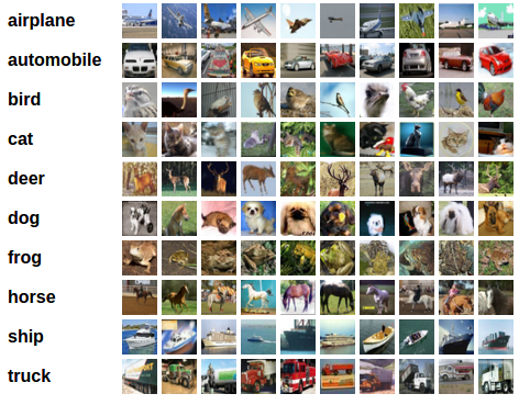
../_static/img/cifar10.png — CIFAR-10 影像示例#

輸入影像是 RGB，因此它們有 3 個通道，大小為 32x32 畫素。基本上，每張影像由 3 x 32 x 32 = 3072 個數字組成，範圍從 0 到 255。在神經網路中，對輸入進行歸一化是一種常見做法，原因有多種，包括避免常用啟用函式的飽和和提高數值穩定性。我們的歸一化過程包括減去每個通道的平均值併除以標準差。張量 “mean=[0.485, 0.456, 0.406]” 和 “std=[0.229, 0.224, 0.225]” 已經計算得出，它們代表了預定義 CIFAR-10 子集中每個通道的平均值和標準差，該子集旨在作為訓練集。請注意，我們也對測試集使用了這些值，而沒有從頭開始重新計算平均值和標準差。這是因為網路是在減去和除以上述數字後產生的特徵上訓練的，我們希望保持一致性。此外，在現實生活中，我們無法計算測試集的平均值和標準差，因為根據我們的假設，此時該資料將無法訪問。

最後一點，我們通常將這個未使用的集合稱為驗證集，在最佳化模型在驗證集上的效能後，我們會使用一個單獨的集合，稱為測試集。這樣做是為了避免基於對單個指標的貪婪和有偏最佳化的模型進行選擇。

# Below we are preprocessing data for CIFAR-10. We use an arbitrary batch size of 128.
transforms_cifar = transforms.Compose([
    transforms.ToTensor(),
    transforms.Normalize(mean=[0.485, 0.456, 0.406], std=[0.229, 0.224, 0.225]),
])

# Loading the CIFAR-10 dataset:
train_dataset = datasets.CIFAR10(root='./data', train=True, download=True, transform=transforms_cifar)
test_dataset = datasets.CIFAR10(root='./data', train=False, download=True, transform=transforms_cifar)

  0%|          | 0.00/170M [00:00<?, ?B/s]
  0%|          | 590k/170M [00:00<00:28, 5.88MB/s]
  4%|▍         | 7.18M/170M [00:00<00:03, 41.0MB/s]
 10%|▉         | 16.4M/170M [00:00<00:02, 63.9MB/s]
 15%|█▌        | 25.6M/170M [00:00<00:01, 75.1MB/s]
 19%|█▉        | 33.2M/170M [00:00<00:01, 71.5MB/s]
 26%|██▌       | 44.4M/170M [00:00<00:01, 84.5MB/s]
 31%|███▏      | 53.6M/170M [00:00<00:01, 86.9MB/s]
 38%|███▊      | 64.2M/170M [00:00<00:01, 92.5MB/s]
 43%|████▎     | 73.6M/170M [00:00<00:01, 93.0MB/s]
 49%|████▊     | 82.9M/170M [00:01<00:00, 93.0MB/s]
 54%|█████▍    | 92.3M/170M [00:01<00:00, 84.2MB/s]
 59%|█████▉    | 101M/170M [00:01<00:00, 83.2MB/s]
 64%|██████▍   | 109M/170M [00:01<00:00, 82.5MB/s]
 69%|██████▉   | 118M/170M [00:01<00:00, 79.9MB/s]
 74%|███████▍  | 126M/170M [00:01<00:00, 81.2MB/s]
 79%|███████▉  | 135M/170M [00:01<00:00, 82.6MB/s]
 85%|████████▍ | 145M/170M [00:01<00:00, 87.4MB/s]
 90%|█████████ | 154M/170M [00:01<00:00, 76.9MB/s]
 95%|█████████▍| 162M/170M [00:02<00:00, 74.9MB/s]
 99%|█████████▉| 169M/170M [00:02<00:00, 74.0MB/s]
100%|██████████| 170M/170M [00:02<00:00, 78.7MB/s]

注意

此部分僅適用於對快速結果感興趣的 CPU 使用者。僅當您對小規模實驗感興趣時才使用此選項。請記住，程式碼應該使用任何 GPU 快速執行。僅從訓練/測試資料集中選擇前 num_images_to_keep 張影像

#from torch.utils.data import Subset
#num_images_to_keep = 2000
#train_dataset = Subset(train_dataset, range(min(num_images_to_keep, 50_000)))
#test_dataset = Subset(test_dataset, range(min(num_images_to_keep, 10_000)))

#Dataloaders
train_loader = torch.utils.data.DataLoader(train_dataset, batch_size=128, shuffle=True, num_workers=2)
test_loader = torch.utils.data.DataLoader(test_dataset, batch_size=128, shuffle=False, num_workers=2)

定義模型類和實用函式#

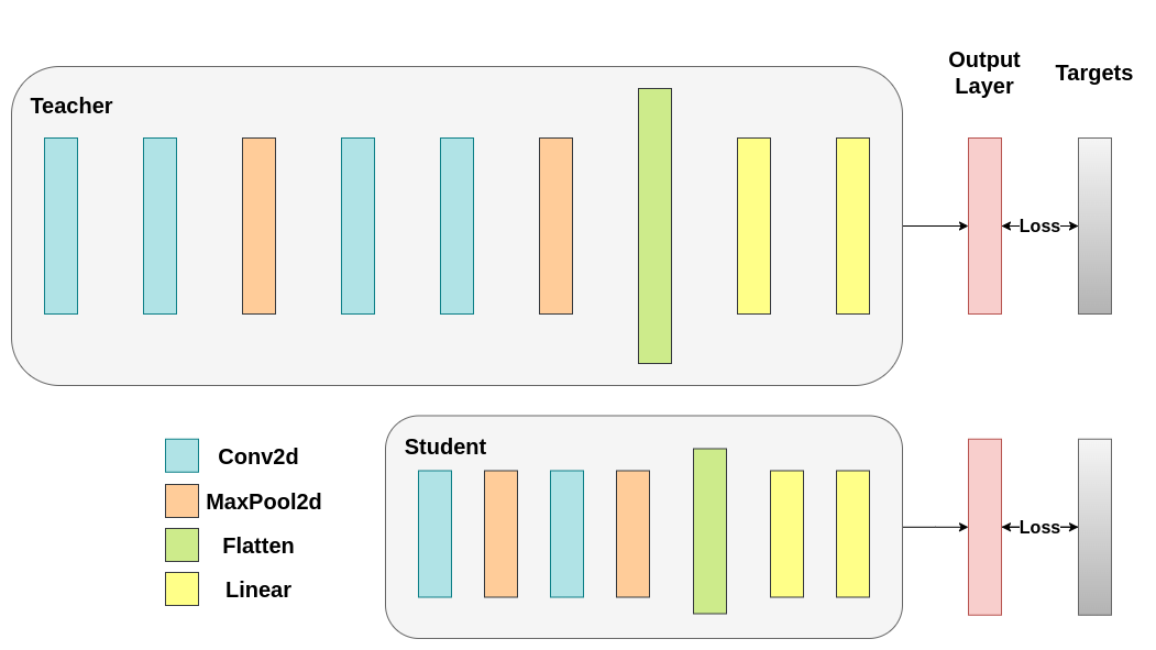
接下來，我們需要定義我們的模型類。這裡需要設定幾個使用者定義的引數。我們使用兩種不同的架構，在我們的實驗中保持濾波器數量固定，以確保公平比較。這兩種架構都是卷積神經網路 (CNN)，具有不同數量的卷積層作為特徵提取器，然後是一個具有 10 個類別的分類器。學生模型的濾波器和神經元數量較少。

# Deeper neural network class to be used as teacher:
class DeepNN(nn.Module):
    def __init__(self, num_classes=10):
        super(DeepNN, self).__init__()
        self.features = nn.Sequential(
            nn.Conv2d(3, 128, kernel_size=3, padding=1),
            nn.ReLU(),
            nn.Conv2d(128, 64, kernel_size=3, padding=1),
            nn.ReLU(),
            nn.MaxPool2d(kernel_size=2, stride=2),
            nn.Conv2d(64, 64, kernel_size=3, padding=1),
            nn.ReLU(),
            nn.Conv2d(64, 32, kernel_size=3, padding=1),
            nn.ReLU(),
            nn.MaxPool2d(kernel_size=2, stride=2),
        )
        self.classifier = nn.Sequential(
            nn.Linear(2048, 512),
            nn.ReLU(),
            nn.Dropout(0.1),
            nn.Linear(512, num_classes)
        )

    def forward(self, x):
        x = self.features(x)
        x = torch.flatten(x, 1)
        x = self.classifier(x)
        return x

# Lightweight neural network class to be used as student:
class LightNN(nn.Module):
    def __init__(self, num_classes=10):
        super(LightNN, self).__init__()
        self.features = nn.Sequential(
            nn.Conv2d(3, 16, kernel_size=3, padding=1),
            nn.ReLU(),
            nn.MaxPool2d(kernel_size=2, stride=2),
            nn.Conv2d(16, 16, kernel_size=3, padding=1),
            nn.ReLU(),
            nn.MaxPool2d(kernel_size=2, stride=2),
        )
        self.classifier = nn.Sequential(
            nn.Linear(1024, 256),
            nn.ReLU(),
            nn.Dropout(0.1),
            nn.Linear(256, num_classes)
        )

    def forward(self, x):
        x = self.features(x)
        x = torch.flatten(x, 1)
        x = self.classifier(x)
        return x

我們使用 2 個函式來幫助我們在原始分類任務上生成和評估結果。一個函式稱為 train，它接受以下引數：

model：一個透過此函式訓練（更新權重）的模型例項。
train_loader：我們上面定義了 train_loader，它的作用是將資料輸入模型。
epochs：我們遍歷資料集的次數。
learning_rate：學習率決定了我們走向收斂的步長有多大。過大或過小的步長都可能有害。
device：確定執行工作負載的裝置。根據可用性，可以是 CPU 或 GPU。

我們的測試函式類似，但它將使用 test_loader 來載入測試集中的影像。

../_static/img/knowledge_distillation/ce_only.png — 使用交叉熵訓練兩個網路。學生模型將用作基線：#

def train(model, train_loader, epochs, learning_rate, device):
    criterion = nn.CrossEntropyLoss()
    optimizer = optim.Adam(model.parameters(), lr=learning_rate)

    model.train()

    for epoch in range(epochs):
        running_loss = 0.0
        for inputs, labels in train_loader:
            # inputs: A collection of batch_size images
            # labels: A vector of dimensionality batch_size with integers denoting class of each image
            inputs, labels = inputs.to(device), labels.to(device)

            optimizer.zero_grad()
            outputs = model(inputs)

            # outputs: Output of the network for the collection of images. A tensor of dimensionality batch_size x num_classes
            # labels: The actual labels of the images. Vector of dimensionality batch_size
            loss = criterion(outputs, labels)
            loss.backward()
            optimizer.step()

            running_loss += loss.item()

        print(f"Epoch {epoch+1}/{epochs}, Loss: {running_loss / len(train_loader)}")

def test(model, test_loader, device):
    model.to(device)
    model.eval()

    correct = 0
    total = 0

    with torch.no_grad():
        for inputs, labels in test_loader:
            inputs, labels = inputs.to(device), labels.to(device)

            outputs = model(inputs)
            _, predicted = torch.max(outputs.data, 1)

            total += labels.size(0)
            correct += (predicted == labels).sum().item()

    accuracy = 100 * correct / total
    print(f"Test Accuracy: {accuracy:.2f}%")
    return accuracy

交叉熵執行#

為了可重現性，我們需要設定 torch 的手動種子。我們使用不同的方法訓練網路，因此為了公平比較，用相同的權重初始化網路是有意義的。首先，使用交叉熵訓練教師網路

torch.manual_seed(42)
nn_deep = DeepNN(num_classes=10).to(device)
train(nn_deep, train_loader, epochs=10, learning_rate=0.001, device=device)
test_accuracy_deep = test(nn_deep, test_loader, device)

# Instantiate the lightweight network:
torch.manual_seed(42)
nn_light = LightNN(num_classes=10).to(device)

Epoch 1/10, Loss: 1.3380480573305389
Epoch 2/10, Loss: 0.8689962590441984
Epoch 3/10, Loss: 0.6735104577773062
Epoch 4/10, Loss: 0.5305723712572357
Epoch 5/10, Loss: 0.4093079611163615
Epoch 6/10, Loss: 0.300734175593042
Epoch 7/10, Loss: 0.21761560725891377
Epoch 8/10, Loss: 0.1718607815959112
Epoch 9/10, Loss: 0.13632688448404717
Epoch 10/10, Loss: 0.11418102288147068
Test Accuracy: 74.84%

我們例項化了一個額外的輕量級網路模型來比較它們的效能。反向傳播對權重初始化很敏感，因此我們需要確保這兩個網路具有完全相同的初始化。

torch.manual_seed(42)
new_nn_light = LightNN(num_classes=10).to(device)

為確保我們建立了第一個網路的副本，我們檢查了其第一層的範數。如果匹配，我們可以安全地得出結論，這兩個網路確實是相同的。

# Print the norm of the first layer of the initial lightweight model
print("Norm of 1st layer of nn_light:", torch.norm(nn_light.features[0].weight).item())
# Print the norm of the first layer of the new lightweight model
print("Norm of 1st layer of new_nn_light:", torch.norm(new_nn_light.features[0].weight).item())

Norm of 1st layer of nn_light: 2.327361822128296
Norm of 1st layer of new_nn_light: 2.327361822128296

列印每個模型中的總引數數量

total_params_deep = "{:,}".format(sum(p.numel() for p in nn_deep.parameters()))
print(f"DeepNN parameters: {total_params_deep}")
total_params_light = "{:,}".format(sum(p.numel() for p in nn_light.parameters()))
print(f"LightNN parameters: {total_params_light}")

DeepNN parameters: 1,186,986
LightNN parameters: 267,738

使用交叉熵損失訓練和測試輕量級網路

train(nn_light, train_loader, epochs=10, learning_rate=0.001, device=device)
test_accuracy_light_ce = test(nn_light, test_loader, device)

Epoch 1/10, Loss: 1.4703684837921807
Epoch 2/10, Loss: 1.1607250258745745
Epoch 3/10, Loss: 1.031156221161718
Epoch 4/10, Loss: 0.931552555554968
Epoch 5/10, Loss: 0.8572665924001532
Epoch 6/10, Loss: 0.7909330646400257
Epoch 7/10, Loss: 0.7265385107311142
Epoch 8/10, Loss: 0.6723965189188642
Epoch 9/10, Loss: 0.6193338737768286
Epoch 10/10, Loss: 0.5720619233825323
Test Accuracy: 70.17%

正如我們所見，基於測試準確性，我們現在可以比較將用作教師的深度網路和我們假定的學生的輕量級網路。到目前為止，我們的學生沒有干預教師，因此這種效能是學生本身實現的。到目前為止的指標可以透過以下幾行看到：

print(f"Teacher accuracy: {test_accuracy_deep:.2f}%")
print(f"Student accuracy: {test_accuracy_light_ce:.2f}%")

Teacher accuracy: 74.84%
Student accuracy: 70.17%

知識蒸餾執行#

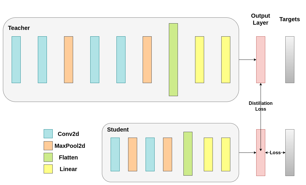
現在讓我們嘗試透過引入教師來提高學生網路的測試準確性。知識蒸餾是一種簡單易行的技術來實現這一目標，基於這樣一個事實：兩個網路都輸出我們類別的機率分佈。因此，兩個網路共享相同數量的輸出神經元。該方法透過在傳統的交叉熵損失中新增一個額外的損失來實現，該損失基於教師網路的 softmax 輸出。假設一個經過適當訓練的教師網路的輸出啟用攜帶了額外資訊，學生網路在訓練過程中可以利用這些資訊。最初的工作表明，利用軟目標中較小機率的比例有助於實現深度神經網路的根本目標，即在資料上建立相似性結構，使相似的物件對映得更近。例如，在 CIFAR-10 中，一輛卡車如果帶有輪子，可能會被誤認為是汽車或飛機，但不太可能被誤認為是狗。因此，假設有價值的資訊不僅存在於經過適當訓練的模型的頂級預測中，還存在於整個輸出分佈中，這是有道理的。然而，僅靠交叉熵不足以充分利用這些資訊，因為非預測類別的啟用往往非常小，以至於傳播的梯度不會有意義地改變權重來構建這種理想的向量空間。

在我們繼續定義第一個引入教師-學生動態的輔助函式時，我們需要包含一些額外的引數：

T：溫度控制輸出分佈的平滑度。較高的 T 會導致更平滑的分佈，從而使較小的機率獲得更大的提升。
soft_target_loss_weight：分配給我們即將包含的額外目標的權重。
ce_loss_weight：分配給交叉熵的權重。調整這些權重會促使網路優先最佳化其中一個目標。

../_static/img/knowledge_distillation/distillation_output_loss.png — 蒸餾損失從網路的 logits 計算得出。它只將梯度返回給學生：#

def train_knowledge_distillation(teacher, student, train_loader, epochs, learning_rate, T, soft_target_loss_weight, ce_loss_weight, device):
    ce_loss = nn.CrossEntropyLoss()
    optimizer = optim.Adam(student.parameters(), lr=learning_rate)

    teacher.eval()  # Teacher set to evaluation mode
    student.train() # Student to train mode

    for epoch in range(epochs):
        running_loss = 0.0
        for inputs, labels in train_loader:
            inputs, labels = inputs.to(device), labels.to(device)

            optimizer.zero_grad()

            # Forward pass with the teacher model - do not save gradients here as we do not change the teacher's weights
            with torch.no_grad():
                teacher_logits = teacher(inputs)

            # Forward pass with the student model
            student_logits = student(inputs)

            #Soften the student logits by applying softmax first and log() second
            soft_targets = nn.functional.softmax(teacher_logits / T, dim=-1)
            soft_prob = nn.functional.log_softmax(student_logits / T, dim=-1)

            # Calculate the soft targets loss. Scaled by T**2 as suggested by the authors of the paper "Distilling the knowledge in a neural network"
            soft_targets_loss = torch.sum(soft_targets * (soft_targets.log() - soft_prob)) / soft_prob.size()[0] * (T**2)

            # Calculate the true label loss
            label_loss = ce_loss(student_logits, labels)

            # Weighted sum of the two losses
            loss = soft_target_loss_weight * soft_targets_loss + ce_loss_weight * label_loss

            loss.backward()
            optimizer.step()

            running_loss += loss.item()

        print(f"Epoch {epoch+1}/{epochs}, Loss: {running_loss / len(train_loader)}")

# Apply ``train_knowledge_distillation`` with a temperature of 2. Arbitrarily set the weights to 0.75 for CE and 0.25 for distillation loss.
train_knowledge_distillation(teacher=nn_deep, student=new_nn_light, train_loader=train_loader, epochs=10, learning_rate=0.001, T=2, soft_target_loss_weight=0.25, ce_loss_weight=0.75, device=device)
test_accuracy_light_ce_and_kd = test(new_nn_light, test_loader, device)

# Compare the student test accuracy with and without the teacher, after distillation
print(f"Teacher accuracy: {test_accuracy_deep:.2f}%")
print(f"Student accuracy without teacher: {test_accuracy_light_ce:.2f}%")
print(f"Student accuracy with CE + KD: {test_accuracy_light_ce_and_kd:.2f}%")

Epoch 1/10, Loss: 2.420701376007646
Epoch 2/10, Loss: 1.9034097984318843
Epoch 3/10, Loss: 1.6752258091021681
Epoch 4/10, Loss: 1.5147676419114213
Epoch 5/10, Loss: 1.3861400674066275
Epoch 6/10, Loss: 1.267950757385215
Epoch 7/10, Loss: 1.1739736123158193
Epoch 8/10, Loss: 1.092016106218938
Epoch 9/10, Loss: 1.0159087505791804
Epoch 10/10, Loss: 0.9451471789718588
Test Accuracy: 71.00%
Teacher accuracy: 74.84%
Student accuracy without teacher: 70.17%
Student accuracy with CE + KD: 71.00%

餘弦損失最小化執行#

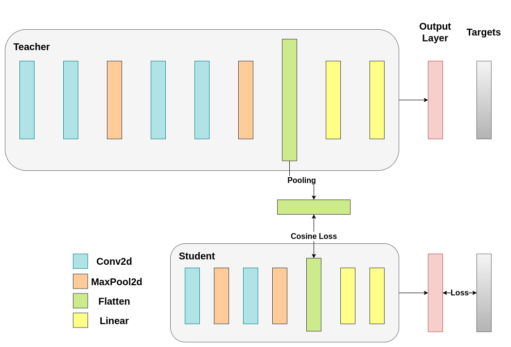
您可以隨意調整控制 softmax 函式平滑度的溫度引數和損失係數。在神經網路中，很容易在主要目標中新增額外的損失函式來實現更好的泛化等目標。讓我們嘗試為學生模型新增一個目標，但現在我們關注它們的隱藏狀態而不是輸出層。我們的目標是透過包含一個樸素的損失函式，將資訊從教師的表示傳遞給學生，該損失函式的最小化意味著扁平化的向量隨後傳遞給分類器，隨著損失的降低，這些向量變得更加“相似”。當然，教師不會更新其權重，因此最小化僅取決於學生的權重。這種方法的原理是我們假設教師模型具有更好的內部表示，學生模型在沒有外部干預的情況下不太可能達到這種表示，因此我們人為地推動學生模仿教師的內部表示。但這是否最終會幫助學生模型並不直接，因為推動輕量級網路達到這一點可能是一件好事，假設我們找到了一個能帶來更好測試準確性的內部表示，但也可能是有害的，因為網路具有不同的架構，學生模型的學習能力不如教師模型。換句話說，這兩個向量（學生和教師的）沒有理由在每個分量上都匹配。學生模型可以達到一個與教師模型表示相置換的內部表示，並且同樣有效。儘管如此，我們仍然可以進行快速實驗來弄清楚這種方法的影響。我們將使用 CosineEmbeddingLoss，其公式如下：

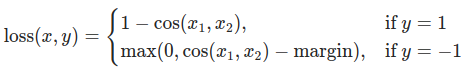
../_static/img/knowledge_distillation/cosine_embedding_loss.png — CosineEmbeddingLoss 公式#

顯然，有一件事需要我們先解決。當我們對輸出層進行蒸餾時，我們提到兩個網路具有相同數量的神經元，等於類別的數量。然而，這對於我們卷積層之後的層來說並非如此。在這裡，在展平最後一個卷積層後，教師擁有的神經元比學生多。我們的損失函式接受兩個維度相同的向量作為輸入，因此我們需要以某種方式匹配它們。我們將透過在教師的卷積層之後包含一個平均池化層來解決這個問題，以減小其維度以匹配學生的維度。

為了繼續，我們將修改我們的模型類，或者建立新的類。現在，forward 函式不僅返回網路的 logits，還返回卷積層之後的扁平化隱藏表示。我們包含了對修改後的教師的上述池化。

class ModifiedDeepNNCosine(nn.Module):
    def __init__(self, num_classes=10):
        super(ModifiedDeepNNCosine, self).__init__()
        self.features = nn.Sequential(
            nn.Conv2d(3, 128, kernel_size=3, padding=1),
            nn.ReLU(),
            nn.Conv2d(128, 64, kernel_size=3, padding=1),
            nn.ReLU(),
            nn.MaxPool2d(kernel_size=2, stride=2),
            nn.Conv2d(64, 64, kernel_size=3, padding=1),
            nn.ReLU(),
            nn.Conv2d(64, 32, kernel_size=3, padding=1),
            nn.ReLU(),
            nn.MaxPool2d(kernel_size=2, stride=2),
        )
        self.classifier = nn.Sequential(
            nn.Linear(2048, 512),
            nn.ReLU(),
            nn.Dropout(0.1),
            nn.Linear(512, num_classes)
        )

    def forward(self, x):
        x = self.features(x)
        flattened_conv_output = torch.flatten(x, 1)
        x = self.classifier(flattened_conv_output)
        flattened_conv_output_after_pooling = torch.nn.functional.avg_pool1d(flattened_conv_output, 2)
        return x, flattened_conv_output_after_pooling

# Create a similar student class where we return a tuple. We do not apply pooling after flattening.
class ModifiedLightNNCosine(nn.Module):
    def __init__(self, num_classes=10):
        super(ModifiedLightNNCosine, self).__init__()
        self.features = nn.Sequential(
            nn.Conv2d(3, 16, kernel_size=3, padding=1),
            nn.ReLU(),
            nn.MaxPool2d(kernel_size=2, stride=2),
            nn.Conv2d(16, 16, kernel_size=3, padding=1),
            nn.ReLU(),
            nn.MaxPool2d(kernel_size=2, stride=2),
        )
        self.classifier = nn.Sequential(
            nn.Linear(1024, 256),
            nn.ReLU(),
            nn.Dropout(0.1),
            nn.Linear(256, num_classes)
        )

    def forward(self, x):
        x = self.features(x)
        flattened_conv_output = torch.flatten(x, 1)
        x = self.classifier(flattened_conv_output)
        return x, flattened_conv_output

# We do not have to train the modified deep network from scratch of course, we just load its weights from the trained instance
modified_nn_deep = ModifiedDeepNNCosine(num_classes=10).to(device)
modified_nn_deep.load_state_dict(nn_deep.state_dict())

# Once again ensure the norm of the first layer is the same for both networks
print("Norm of 1st layer for deep_nn:", torch.norm(nn_deep.features[0].weight).item())
print("Norm of 1st layer for modified_deep_nn:", torch.norm(modified_nn_deep.features[0].weight).item())

# Initialize a modified lightweight network with the same seed as our other lightweight instances. This will be trained from scratch to examine the effectiveness of cosine loss minimization.
torch.manual_seed(42)
modified_nn_light = ModifiedLightNNCosine(num_classes=10).to(device)
print("Norm of 1st layer:", torch.norm(modified_nn_light.features[0].weight).item())

Norm of 1st layer for deep_nn: 7.468933582305908
Norm of 1st layer for modified_deep_nn: 7.468933582305908
Norm of 1st layer: 2.327361822128296

自然，我們需要為此更改訓練迴圈，因為現在模型返回一個元組 (logits, hidden_representation)。使用樣本輸入張量，我們可以列印它們的形狀。

# Create a sample input tensor
sample_input = torch.randn(128, 3, 32, 32).to(device) # Batch size: 128, Filters: 3, Image size: 32x32

# Pass the input through the student
logits, hidden_representation = modified_nn_light(sample_input)

# Print the shapes of the tensors
print("Student logits shape:", logits.shape) # batch_size x total_classes
print("Student hidden representation shape:", hidden_representation.shape) # batch_size x hidden_representation_size

# Pass the input through the teacher
logits, hidden_representation = modified_nn_deep(sample_input)

# Print the shapes of the tensors
print("Teacher logits shape:", logits.shape) # batch_size x total_classes
print("Teacher hidden representation shape:", hidden_representation.shape) # batch_size x hidden_representation_size

Student logits shape: torch.Size([128, 10])
Student hidden representation shape: torch.Size([128, 1024])
Teacher logits shape: torch.Size([128, 10])
Teacher hidden representation shape: torch.Size([128, 1024])

在我們的例子中，hidden_representation_size 是 1024。這是學生模型的最後一個卷積層的扁平化特徵圖，正如您所見，它是其分類器的輸入。對於教師模型，它也是 1024，因為我們透過 avg_pool1d 從 2048 進行了設定。這裡應用的損失僅影響學生模型在損失計算之前的權重。換句話說，它不影響學生模型的分類器。修改後的訓練迴圈如下：

../_static/img/knowledge_distillation/cosine_loss_distillation.png — 在餘弦損失最小化中，我們希望透過將梯度返回給學生來最大化兩個表示的餘弦相似度：#

def train_cosine_loss(teacher, student, train_loader, epochs, learning_rate, hidden_rep_loss_weight, ce_loss_weight, device):
    ce_loss = nn.CrossEntropyLoss()
    cosine_loss = nn.CosineEmbeddingLoss()
    optimizer = optim.Adam(student.parameters(), lr=learning_rate)

    teacher.to(device)
    student.to(device)
    teacher.eval()  # Teacher set to evaluation mode
    student.train() # Student to train mode

    for epoch in range(epochs):
        running_loss = 0.0
        for inputs, labels in train_loader:
            inputs, labels = inputs.to(device), labels.to(device)

            optimizer.zero_grad()

            # Forward pass with the teacher model and keep only the hidden representation
            with torch.no_grad():
                _, teacher_hidden_representation = teacher(inputs)

            # Forward pass with the student model
            student_logits, student_hidden_representation = student(inputs)

            # Calculate the cosine loss. Target is a vector of ones. From the loss formula above we can see that is the case where loss minimization leads to cosine similarity increase.
            hidden_rep_loss = cosine_loss(student_hidden_representation, teacher_hidden_representation, target=torch.ones(inputs.size(0)).to(device))

            # Calculate the true label loss
            label_loss = ce_loss(student_logits, labels)

            # Weighted sum of the two losses
            loss = hidden_rep_loss_weight * hidden_rep_loss + ce_loss_weight * label_loss

            loss.backward()
            optimizer.step()

            running_loss += loss.item()

        print(f"Epoch {epoch+1}/{epochs}, Loss: {running_loss / len(train_loader)}")

出於相同的原因，我們需要修改我們的測試函式。這裡我們忽略模型返回的隱藏表示。

def test_multiple_outputs(model, test_loader, device):
    model.to(device)
    model.eval()

    correct = 0
    total = 0

    with torch.no_grad():
        for inputs, labels in test_loader:
            inputs, labels = inputs.to(device), labels.to(device)

            outputs, _ = model(inputs) # Disregard the second tensor of the tuple
            _, predicted = torch.max(outputs.data, 1)

            total += labels.size(0)
            correct += (predicted == labels).sum().item()

    accuracy = 100 * correct / total
    print(f"Test Accuracy: {accuracy:.2f}%")
    return accuracy

在這種情況下，我們可以輕鬆地將知識蒸餾和餘弦損失最小化都包含在一個函式中。通常會結合使用多種方法來實現教師-學生正規化中的更好效能。目前，我們可以執行一個簡單的訓練-測試會話。

# Train and test the lightweight network with cross entropy loss
train_cosine_loss(teacher=modified_nn_deep, student=modified_nn_light, train_loader=train_loader, epochs=10, learning_rate=0.001, hidden_rep_loss_weight=0.25, ce_loss_weight=0.75, device=device)
test_accuracy_light_ce_and_cosine_loss = test_multiple_outputs(modified_nn_light, test_loader, device)

Epoch 1/10, Loss: 1.3003839559262367
Epoch 2/10, Loss: 1.0687231790379186
Epoch 3/10, Loss: 0.9705146174601582
Epoch 4/10, Loss: 0.8942109386024573
Epoch 5/10, Loss: 0.8398711993871137
Epoch 6/10, Loss: 0.7960785875844834
Epoch 7/10, Loss: 0.7546686552979452
Epoch 8/10, Loss: 0.7190434603435
Epoch 9/10, Loss: 0.6790954071237608
Epoch 10/10, Loss: 0.6566963798707098
Test Accuracy: 70.60%

中間迴歸器執行#

我們的樸素最小化不能保證更好的結果，原因有幾個，其中之一是向量的維度。對於更高維度的向量，餘弦相似度通常比歐幾里得距離效果更好，但我們處理的是每個向量有 1024 個分量，因此提取有意義的相似度要困難得多。此外，正如我們提到的，推動匹配教師和學生的隱藏表示不受理論支援。我們沒有充分的理由去追求這些向量的一對一匹配。我們將透過引入一個名為迴歸器的額外網路來提供一個最終的訓練干預示例。目標是首先提取教師在卷積層之後的特徵圖，然後提取學生在卷積層之後的特徵圖，最後嘗試匹配這些圖。然而，這次，我們將在網路之間引入一個迴歸器來促進匹配過程。迴歸器是可訓練的，並且理想情況下會比我們的樸素餘弦損失最小化方案做得更好。它的主要工作是匹配這些特徵圖的維度，以便我們可以正確地定義教師和學生之間的損失函式。定義這樣一個損失函式提供了一個教學“路徑”，這基本上是一個用於反向傳播梯度以改變學生權重的流。關注我們原始網路分類器之前的卷積層的輸出，我們有以下形狀：

# Pass the sample input only from the convolutional feature extractor
convolutional_fe_output_student = nn_light.features(sample_input)
convolutional_fe_output_teacher = nn_deep.features(sample_input)

# Print their shapes
print("Student's feature extractor output shape: ", convolutional_fe_output_student.shape)
print("Teacher's feature extractor output shape: ", convolutional_fe_output_teacher.shape)

Student's feature extractor output shape:  torch.Size([128, 16, 8, 8])
Teacher's feature extractor output shape:  torch.Size([128, 32, 8, 8])

教師有 32 個濾波器，學生有 16 個濾波器。我們將包括一個可訓練層，該層將學生模型的特徵圖轉換為教師模型特徵圖的形狀。實際上，我們修改輕量級模型以返回中間迴歸器之後的隱藏狀態，該回歸器匹配卷積特徵圖的尺寸，並修改教師模型以返回最終卷積層之後的輸出，而無需池化或展平。

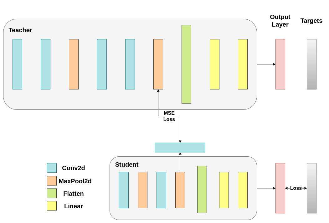
../_static/img/knowledge_distillation/fitnets_knowledge_distill.png — 可訓練層匹配中間張量的形狀，並且均方誤差 (MSE) 被正確定義：#

class ModifiedDeepNNRegressor(nn.Module):
    def __init__(self, num_classes=10):
        super(ModifiedDeepNNRegressor, self).__init__()
        self.features = nn.Sequential(
            nn.Conv2d(3, 128, kernel_size=3, padding=1),
            nn.ReLU(),
            nn.Conv2d(128, 64, kernel_size=3, padding=1),
            nn.ReLU(),
            nn.MaxPool2d(kernel_size=2, stride=2),
            nn.Conv2d(64, 64, kernel_size=3, padding=1),
            nn.ReLU(),
            nn.Conv2d(64, 32, kernel_size=3, padding=1),
            nn.ReLU(),
            nn.MaxPool2d(kernel_size=2, stride=2),
        )
        self.classifier = nn.Sequential(
            nn.Linear(2048, 512),
            nn.ReLU(),
            nn.Dropout(0.1),
            nn.Linear(512, num_classes)
        )

    def forward(self, x):
        x = self.features(x)
        conv_feature_map = x
        x = torch.flatten(x, 1)
        x = self.classifier(x)
        return x, conv_feature_map

class ModifiedLightNNRegressor(nn.Module):
    def __init__(self, num_classes=10):
        super(ModifiedLightNNRegressor, self).__init__()
        self.features = nn.Sequential(
            nn.Conv2d(3, 16, kernel_size=3, padding=1),
            nn.ReLU(),
            nn.MaxPool2d(kernel_size=2, stride=2),
            nn.Conv2d(16, 16, kernel_size=3, padding=1),
            nn.ReLU(),
            nn.MaxPool2d(kernel_size=2, stride=2),
        )
        # Include an extra regressor (in our case linear)
        self.regressor = nn.Sequential(
            nn.Conv2d(16, 32, kernel_size=3, padding=1)
        )
        self.classifier = nn.Sequential(
            nn.Linear(1024, 256),
            nn.ReLU(),
            nn.Dropout(0.1),
            nn.Linear(256, num_classes)
        )

    def forward(self, x):
        x = self.features(x)
        regressor_output = self.regressor(x)
        x = torch.flatten(x, 1)
        x = self.classifier(x)
        return x, regressor_output

之後，我們必須再次更新我們的訓練迴圈。這次，我們提取學生的迴歸器輸出、教師模型的特徵圖，我們計算這些張量上的 MSE（它們具有完全相同的形狀，因此正確定義），並且我們基於該損失進行反向傳播梯度，此外還有分類任務的常規交叉熵損失。

def train_mse_loss(teacher, student, train_loader, epochs, learning_rate, feature_map_weight, ce_loss_weight, device):
    ce_loss = nn.CrossEntropyLoss()
    mse_loss = nn.MSELoss()
    optimizer = optim.Adam(student.parameters(), lr=learning_rate)

    teacher.to(device)
    student.to(device)
    teacher.eval()  # Teacher set to evaluation mode
    student.train() # Student to train mode

    for epoch in range(epochs):
        running_loss = 0.0
        for inputs, labels in train_loader:
            inputs, labels = inputs.to(device), labels.to(device)

            optimizer.zero_grad()

            # Again ignore teacher logits
            with torch.no_grad():
                _, teacher_feature_map = teacher(inputs)

            # Forward pass with the student model
            student_logits, regressor_feature_map = student(inputs)

            # Calculate the loss
            hidden_rep_loss = mse_loss(regressor_feature_map, teacher_feature_map)

            # Calculate the true label loss
            label_loss = ce_loss(student_logits, labels)

            # Weighted sum of the two losses
            loss = feature_map_weight * hidden_rep_loss + ce_loss_weight * label_loss

            loss.backward()
            optimizer.step()

            running_loss += loss.item()

        print(f"Epoch {epoch+1}/{epochs}, Loss: {running_loss / len(train_loader)}")

# Notice how our test function remains the same here with the one we used in our previous case. We only care about the actual outputs because we measure accuracy.

# Initialize a ModifiedLightNNRegressor
torch.manual_seed(42)
modified_nn_light_reg = ModifiedLightNNRegressor(num_classes=10).to(device)

# We do not have to train the modified deep network from scratch of course, we just load its weights from the trained instance
modified_nn_deep_reg = ModifiedDeepNNRegressor(num_classes=10).to(device)
modified_nn_deep_reg.load_state_dict(nn_deep.state_dict())

# Train and test once again
train_mse_loss(teacher=modified_nn_deep_reg, student=modified_nn_light_reg, train_loader=train_loader, epochs=10, learning_rate=0.001, feature_map_weight=0.25, ce_loss_weight=0.75, device=device)
test_accuracy_light_ce_and_mse_loss = test_multiple_outputs(modified_nn_light_reg, test_loader, device)

Epoch 1/10, Loss: 1.7872563826153651
Epoch 2/10, Loss: 1.3899962301449398
Epoch 3/10, Loss: 1.2393632121098317
Epoch 4/10, Loss: 1.1407289636104614
Epoch 5/10, Loss: 1.0597244144400673
Epoch 6/10, Loss: 0.997323940781986
Epoch 7/10, Loss: 0.94199667242177
Epoch 8/10, Loss: 0.8927582682246138
Epoch 9/10, Loss: 0.8498489679887776
Epoch 10/10, Loss: 0.8145248348755605
Test Accuracy: 71.04%

預計最終方法將比 CosineLoss 效果更好，因為現在我們在教師和學生之間允許了一個可訓練層，這給了學生在學習方面一定的靈活性，而不是迫使學生複製教師的表示。包含額外的網路是基於提示的蒸餾的思想。

print(f"Teacher accuracy: {test_accuracy_deep:.2f}%")
print(f"Student accuracy without teacher: {test_accuracy_light_ce:.2f}%")
print(f"Student accuracy with CE + KD: {test_accuracy_light_ce_and_kd:.2f}%")
print(f"Student accuracy with CE + CosineLoss: {test_accuracy_light_ce_and_cosine_loss:.2f}%")
print(f"Student accuracy with CE + RegressorMSE: {test_accuracy_light_ce_and_mse_loss:.2f}%")

Teacher accuracy: 74.84%
Student accuracy without teacher: 70.17%
Student accuracy with CE + KD: 71.00%
Student accuracy with CE + CosineLoss: 70.60%
Student accuracy with CE + RegressorMSE: 71.04%

結論#

上述任何方法都不會增加網路的引數數量或推理時間，因此效能的提高是以在訓練期間計算梯度的微小成本為代價的。在 ML 應用中，我們主要關心推理時間，因為訓練發生在模型部署之前。如果我們的輕量級模型對於部署來說仍然太重，我們可以應用不同的想法，例如訓練後量化。額外的損失可以應用於許多工，而不僅僅是分類，您可以嘗試調整係數、溫度或神經元數量等數量。您可以隨意調整教程中的任何數字，但請記住，如果您更改神經元/濾波器的數量，很可能會發生形狀不匹配。

有關更多資訊，請參閱

指令碼總執行時間： (4 分鐘 7.411 秒)