advanced/semi_structured_sparse

在 Google Colab 中執行

Colab

下載 Notebook

Notebook

在 GitHub 上檢視

GitHub

(beta) 使用半結構化（2:4）稀疏性加速 BERT

創建於：2024 年 4 月 22 日 | 最後更新：2025 年 9 月 29 日 | 最後驗證：2024 年 11 月 5 日

作者：Jesse Cai

概述

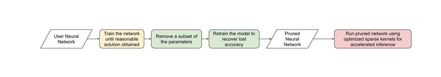
與其他形式的稀疏性一樣，半結構化稀疏性是一種模型最佳化技術，旨在以犧牲一些模型準確性為代價來減少神經網路的記憶體開銷和延遲。它也稱為細粒度結構化稀疏性或2:4 結構化稀疏性。

半結構化稀疏性的名稱來源於其獨特的稀疏模式，即每 2n 個元素中修剪 n 個。我們最常看到 n=2，因此是 2:4 稀疏性。半結構化稀疏性特別有趣，因為它可以在 GPU 上高效加速，並且不會像其他稀疏模式那樣顯著降低模型準確性。

透過引入半結構化稀疏性支援，無需離開 PyTorch 即可修剪和加速半結構化稀疏模型。本教程將對此過程進行說明。

在本教程結束時，我們將一個 BERT 問答模型稀疏化為 2:4 稀疏，並對其進行微調，以恢復幾乎所有 F1 損失（86.92 密集 vs 86.48 稀疏）。最後，我們將加速這個 2:4 稀疏模型進行推理，從而提高 1.3 倍的速度。

要求

• PyTorch >= 2.1。

• 支援半結構化稀疏性的 NVIDIA GPU（計算能力 8.0+）。

注意

本教程在 NVIDIA A100 80GB GPU 上進行了測試。您可能不會在較新的 GPU 架構上看到類似的速度提升。有關半結構化稀疏性支援的最新資訊，請參閱`這裡的 README <pytorch/ao>

本教程專為半結構化稀疏性和一般稀疏性的初學者設計。對於已擁有 2:4 稀疏模型的使用者，使用 to_sparse_semi_structured 加速 nn.Linear 層進行推理非常直接。這是一個示例

import torch
from torch.sparse import to_sparse_semi_structured, SparseSemiStructuredTensor
from torch.utils.benchmark import Timer

# mask Linear weight to be 2:4 sparse
mask = torch.Tensor([0, 0, 1, 1]).tile((3072, 2560)).cuda().bool()
linear = torch.nn.Linear(10240, 3072).half().cuda().eval()
linear.weight = torch.nn.Parameter(mask * linear.weight)

x = torch.rand(3072, 10240).half().cuda()

with torch.inference_mode():
    dense_output = linear(x)
    dense_t = Timer(stmt="linear(x)",
                    globals={"linear": linear,
                             "x": x}).blocked_autorange().median * 1e3

    # accelerate via SparseSemiStructuredTensor
    linear.weight = torch.nn.Parameter(to_sparse_semi_structured(linear.weight))

    sparse_output = linear(x)
    sparse_t = Timer(stmt="linear(x)",
                    globals={"linear": linear,
                             "x": x}).blocked_autorange().median * 1e3

    # sparse and dense matmul are numerically equivalent
    # On an A100 80GB, we see: `Dense: 0.870ms Sparse: 0.630ms | Speedup: 1.382x`
    assert torch.allclose(sparse_output, dense_output, atol=1e-3)
    print(f"Dense: {dense_t:.3f}ms Sparse: {sparse_t:.3f}ms | Speedup: {(dense_t / sparse_t):.3f}x")

半結構化稀疏性解決了什麼問題？

稀疏性的總體動機很簡單：如果網路中有零，您可以透過不儲存或計算這些引數來最佳化效率。然而，稀疏性的具體細節很棘手。將引數歸零並不會立即影響我們模型的延遲/記憶體開銷。

這是因為密集張量仍然包含被修剪（零）的元素，密集矩陣乘法核心仍將在此元素上進行操作。為了實現效能提升，我們需要用稀疏核心替換密集核心，稀疏核心會跳過涉及被修剪元素的計算。

為此，這些核心處理稀疏矩陣，稀疏矩陣不儲存被修剪的元素，並以壓縮格式儲存指定的元素。

對於半結構化稀疏性，我們儲存原始引數的精確一半，以及關於元素排列方式的一些壓縮元資料。

有許多不同的稀疏佈局，每種佈局都有其優點和缺點。2:4 半結構化稀疏佈局特別有趣，原因有兩個：

• 與以前的稀疏格式不同，半結構化稀疏性被設計為可以在 GPU 上高效加速。2020 年，NVIDIA 在其 Ampere 架構中引入了對半結構化稀疏性的硬體支援，並透過 CUTLASS cuSPARSELt 釋出了快速稀疏核心。

• 同時，與其他稀疏格式相比，半結構化稀疏性對模型準確性的影響往往較小，特別是當考慮更高階的修剪/微調方法時。NVIDIA 在其白皮書中表明，一次簡單的幅度修剪至 2:4 稀疏然後重新訓練模型的正規化可以產生幾乎相同的模型準確性。

半結構化稀疏性處於一個最佳點，在較低的稀疏度（50%）下提供 2 倍（理論）的速度提升，同時仍然足夠精細以保持模型準確性。

網路	資料集	指標	密集 FP16	稀疏 FP16
ResNet-50	ImageNet	Top-1	76.1	76.2
ResNeXt-101_32x8d	ImageNet	Top-1	79.3	79.3
Xception	ImageNet	Top-1	79.2	79.2
SSD-RN50	COCO2017	bbAP	24.8	24.8
MaskRCNN-RN50	COCO2017	bbAP	37.9	37.9
FairSeq Transformer	EN-DE WMT14	BLEU	28.2	28.5
BERT-Large	SQuAD v1.1	F1	91.9	91.9

從工作流程的角度來看，半結構化稀疏性還有一個額外的優勢。由於稀疏度固定為 50%，因此更容易將模型稀疏化的問題分解為兩個不同的子問題：

• 準確性 - 如何找到一組 2:4 稀疏權重，以最大程度地減少我們模型的準確性下降？

• 效能 - 如何加速我們的 2:4 稀疏權重以進行推理並減少記憶體開銷？

\[\begin{bmatrix} 1 & 1 & 0 & 0 \\ 0 & 0 & 1 & 1 \\ 1 & 0 & 0 & 0 \\ 0 & 0 & 1 & 1 \\ \end{bmatrix}\]

這些問題之間的自然交接點是歸零的密集張量。我們的推理解決方案旨在以這種格式壓縮和加速張量。我們預計許多使用者將提出自定義掩蔽解決方案，因為這是一個活躍的研究領域。

現在我們對半結構化稀疏性有了更多的瞭解，讓我們將其應用於在問答任務 SQuAD 上訓練的 BERT 模型。

簡介與設定

讓我們開始匯入所有需要的包。

# If you are running this in Google Colab, run:
# .. code-block: python
#
#    !pip install datasets transformers evaluate accelerate pandas
#
import os
os.environ["WANDB_DISABLED"] = "true"

import collections
import datasets
import evaluate
import numpy as np
import torch
import torch.utils.benchmark as benchmark
from torch import nn
from torch.sparse import to_sparse_semi_structured, SparseSemiStructuredTensor
from torch.ao.pruning import WeightNormSparsifier
import transformers

# force CUTLASS use if ``cuSPARSELt`` is not available
torch.manual_seed(100)

# Set default device to "cuda:0"
torch.set_default_device(torch.device("cuda:0" if torch.cuda.is_available() else "cpu"))

我們還需要定義一些特定於當前資料集/任務的輔助函式。這些函式改編自這個 Hugging Face 課程作為參考。

def preprocess_validation_function(examples, tokenizer):
    inputs = tokenizer(
        [q.strip() for q in examples["question"]],
        examples["context"],
        max_length=384,
        truncation="only_second",
        return_overflowing_tokens=True,
        return_offsets_mapping=True,
        padding="max_length",
    )
    sample_map = inputs.pop("overflow_to_sample_mapping")
    example_ids = []

    for i in range(len(inputs["input_ids"])):
        sample_idx = sample_map[i]
        example_ids.append(examples["id"][sample_idx])
        sequence_ids = inputs.sequence_ids(i)
        offset = inputs["offset_mapping"][i]
        inputs["offset_mapping"][i] = [
            o if sequence_ids[k] == 1 else None for k, o in enumerate(offset)
        ]

    inputs["example_id"] = example_ids
    return inputs


def preprocess_train_function(examples, tokenizer):
    inputs = tokenizer(
        [q.strip() for q in examples["question"]],
        examples["context"],
        max_length=384,
        truncation="only_second",
        return_offsets_mapping=True,
        padding="max_length",
    )

    offset_mapping = inputs["offset_mapping"]
    answers = examples["answers"]
    start_positions = []
    end_positions = []

    for i, (offset, answer) in enumerate(zip(offset_mapping, answers)):
        start_char = answer["answer_start"][0]
        end_char = start_char + len(answer["text"][0])
        sequence_ids = inputs.sequence_ids(i)

        # Find the start and end of the context
        idx = 0
        while sequence_ids[idx] != 1:
            idx += 1
        context_start = idx
        while sequence_ids[idx] == 1:
            idx += 1
        context_end = idx - 1

        # If the answer is not fully inside the context, label it (0, 0)
        if offset[context_start][0] > end_char or offset[context_end][1] < start_char:
            start_positions.append(0)
            end_positions.append(0)
        else:
            # Otherwise it's the start and end token positions
            idx = context_start
            while idx <= context_end and offset[idx][0] <= start_char:
                idx += 1
            start_positions.append(idx - 1)

            idx = context_end
            while idx >= context_start and offset[idx][1] >= end_char:
                idx -= 1
            end_positions.append(idx + 1)

    inputs["start_positions"] = start_positions
    inputs["end_positions"] = end_positions
    return inputs


def compute_metrics(start_logits, end_logits, features, examples):
    n_best = 20
    max_answer_length = 30
    metric = evaluate.load("squad")

    example_to_features = collections.defaultdict(list)
    for idx, feature in enumerate(features):
        example_to_features[feature["example_id"]].append(idx)

    predicted_answers = []
    # for example in ``tqdm`` (examples):
    for example in examples:
        example_id = example["id"]
        context = example["context"]
        answers = []

        # Loop through all features associated with that example
        for feature_index in example_to_features[example_id]:
            start_logit = start_logits[feature_index]
            end_logit = end_logits[feature_index]
            offsets = features[feature_index]["offset_mapping"]

            start_indexes = np.argsort(start_logit)[-1 : -n_best - 1 : -1].tolist()
            end_indexes = np.argsort(end_logit)[-1 : -n_best - 1 : -1].tolist()
            for start_index in start_indexes:
                for end_index in end_indexes:
                    # Skip answers that are not fully in the context
                    if offsets[start_index] is None or offsets[end_index] is None:
                        continue
                    # Skip answers with a length that is either < 0
                    # or > max_answer_length
                    if (
                        end_index < start_index
                        or end_index - start_index + 1 > max_answer_length
                    ):
                        continue

                    answer = {
                        "text": context[
                            offsets[start_index][0] : offsets[end_index][1]
                        ],
                        "logit_score": start_logit[start_index] + end_logit[end_index],
                    }
                    answers.append(answer)

        # Select the answer with the best score
        if len(answers) > 0:
            best_answer = max(answers, key=lambda x: x["logit_score"])
            predicted_answers.append(
                {"id": example_id, "prediction_text": best_answer["text"]}
            )
        else:
            predicted_answers.append({"id": example_id, "prediction_text": ""})

    theoretical_answers = [
        {"id": ex["id"], "answers": ex["answers"]} for ex in examples
    ]
    return metric.compute(predictions=predicted_answers, references=theoretical_answers)

在定義了這些函式之後，我們只需要一個額外的輔助函式，它將幫助我們對模型進行基準測試。

def measure_execution_time(model, batch_sizes, dataset):
    dataset_for_model = dataset.remove_columns(["example_id", "offset_mapping"])
    dataset_for_model.set_format("torch")
    batch_size_to_time_sec = {}
    for batch_size in batch_sizes:
        batch = {
            k: dataset_for_model[k][:batch_size].cuda()
            for k in dataset_for_model.column_names
        }

        with torch.no_grad():
            baseline_predictions = model(**batch)
            timer = benchmark.Timer(
                stmt="model(**batch)", globals={"model": model, "batch": batch}
            )
            p50 = timer.blocked_autorange().median * 1000
            batch_size_to_time_sec[batch_size] = p50

            model_c = torch.compile(model, fullgraph=True)
            timer = benchmark.Timer(
                stmt="model(**batch)", globals={"model": model_c, "batch": batch}
            )
            p50 = timer.blocked_autorange().median * 1000
            batch_size_to_time_sec[f"{batch_size}_compile"] = p50
            new_predictions = model_c(**batch)

    return batch_size_to_time_sec

我們將從載入模型和分詞器開始，然後設定我們的資料集。

# load model
model_name = "bert-base-cased"
tokenizer = transformers.AutoTokenizer.from_pretrained(model_name)
model = transformers.AutoModelForQuestionAnswering.from_pretrained(model_name)
print(f"Loading tokenizer: {model_name}")
print(f"Loading model: {model_name}")

# set up train and val dataset
squad_dataset = datasets.load_dataset("squad")
tokenized_squad_dataset = {}
tokenized_squad_dataset["train"] = squad_dataset["train"].map(
    lambda x: preprocess_train_function(x, tokenizer), batched=True
)
tokenized_squad_dataset["validation"] = squad_dataset["validation"].map(
    lambda x: preprocess_validation_function(x, tokenizer),
    batched=True,
    remove_columns=squad_dataset["train"].column_names,
)
data_collator = transformers.DataCollatorWithPadding(tokenizer=tokenizer)

建立基線

接下來，我們將對我們的 BERT 模型在 SQuAD 上進行快速基線訓練。此任務要求模型識別給定上下文中（維基百科文章）回答給定問題的文字片段或段落。執行以下程式碼，我得到了 86.9 的 F1 分數。這非常接近 NVIDIA 報告的分數，差異可能歸因於 BERT-base 與 BERT-large 或微調的超引數。

training_args = transformers.TrainingArguments(
    "trainer",
    num_train_epochs=1,
    lr_scheduler_type="constant",
    per_device_train_batch_size=32,
    per_device_eval_batch_size=256,
    logging_steps=50,
    # Limit max steps for tutorial runners. Delete the below line to see the reported accuracy numbers.
    max_steps=500,
    report_to=None,
)

trainer = transformers.Trainer(
    model,
    training_args,
    train_dataset=tokenized_squad_dataset["train"],
    eval_dataset=tokenized_squad_dataset["validation"],
    data_collator=data_collator,
    tokenizer=tokenizer,
)

trainer.train()

# batch sizes to compare for eval
batch_sizes = [4, 16, 64, 256]
# 2:4 sparsity require fp16, so we cast here for a fair comparison
with torch.autocast("cuda"):
    with torch.no_grad():
        predictions = trainer.predict(tokenized_squad_dataset["validation"])
        start_logits, end_logits = predictions.predictions
        fp16_baseline = compute_metrics(
            start_logits,
            end_logits,
            tokenized_squad_dataset["validation"],
            squad_dataset["validation"],
        )
        fp16_time = measure_execution_time(
            model,
            batch_sizes,
            tokenized_squad_dataset["validation"],
        )

print("fp16", fp16_baseline)
print("cuda_fp16 time", fp16_time)

import pandas as pd
df = pd.DataFrame(trainer.state.log_history)
df.plot.line(x='step', y='loss', title="Loss vs. # steps", ylabel="loss")

將 BERT 修剪為 2:4 稀疏

現在我們有了基線，是時候修剪 BERT 了。有許多不同的修剪策略，但最常見的策略之一是幅度修剪，旨在移除 L1 範數最小的權重。NVIDIA 在其所有結果中都使用了幅度修剪，並且它是一個常見的基線。

為此，我們將使用 torch.ao.pruning 包，其中包含一個權重範數（幅度）稀疏器。這些稀疏器透過將掩碼引數化應用於模型的權重張量來工作。這使它們能夠透過掩蔽被修剪的權重來模擬稀疏性。

我們還必須決定要對模型的哪些層應用稀疏性，在本例中是所有 nn.Linear 層，但特定於任務的輸出頭除外。這是因為半結構化稀疏性有形狀約束，而特定於任務的 nn.Linear 層不滿足這些約束。

sparsifier = WeightNormSparsifier(
    # apply sparsity to all blocks
    sparsity_level=1.0,
    # shape of 4 elements is a block
    sparse_block_shape=(1, 4),
    # two zeros for every block of 4
    zeros_per_block=2
)

# add to config if ``nn.Linear`` and in the BERT model.
sparse_config = [
    {"tensor_fqn": f"{fqn}.weight"}
    for fqn, module in model.named_modules()
    if isinstance(module, nn.Linear) and "layer" in fqn
]

修剪模型的第一個步驟是插入引數化以掩蔽模型的權重。這透過 prepare 步驟完成。任何時候我們嘗試訪問 .weight，我們將得到 mask * weight。

# Prepare the model, insert fake-sparsity parametrizations for training
sparsifier.prepare(model, sparse_config)
print(model.bert.encoder.layer[0].output)

然後，我們將進行一次修剪。所有修剪器都實現了一個 update_mask() 方法，該方法根據修剪器的實現邏輯更新掩碼。step 方法會為稀疏配置中指定的權重呼叫此 update_mask 函式。

我們還將評估模型，以顯示零樣本修剪（即不進行微調/重新訓練的修剪）的準確性下降。

sparsifier.step()
with torch.autocast("cuda"):
    with torch.no_grad():
        predictions = trainer.predict(tokenized_squad_dataset["validation"])
    pruned = compute_metrics(
        *predictions.predictions,
        tokenized_squad_dataset["validation"],
        squad_dataset["validation"],
    )
print("pruned eval metrics:", pruned)

在此狀態下，我們可以開始微調模型，更新不會被修剪的元素，以更好地彌補準確性損失。一旦達到滿意狀態，我們就可以呼叫 squash_mask 來融合掩碼和權重。這將移除引數化，我們留下一個歸零的 2:4 密集模型。

trainer.train()
sparsifier.squash_mask()
torch.set_printoptions(edgeitems=4)
print(model.bert.encoder.layer[0].intermediate.dense.weight[:8, :8])

df["sparse_loss"] = pd.DataFrame(trainer.state.log_history)["loss"]
df.plot.line(x='step', y=["loss", "sparse_loss"], title="Loss vs. # steps", ylabel="loss")

加速 2:4 稀疏模型進行推理

現在我們有了一個這種格式的模型，我們可以像在 QuickStart 指南中一樣加速它進行推理。

model = model.cuda().half()
# accelerate for sparsity
for fqn, module in model.named_modules():
    if isinstance(module, nn.Linear) and "layer" in fqn:
        module.weight = nn.Parameter(to_sparse_semi_structured(module.weight))

with torch.no_grad():
    predictions = trainer.predict(tokenized_squad_dataset["validation"])
start_logits, end_logits = predictions.predictions
metrics_sparse = compute_metrics(
    start_logits,
    end_logits,
    tokenized_squad_dataset["validation"],
    squad_dataset["validation"],
)
print("sparse eval metrics: ", metrics_sparse)
sparse_perf = measure_execution_time(
    model,
    batch_sizes,
    tokenized_squad_dataset["validation"],
)
print("sparse perf metrics: ", sparse_perf)

在幅度修剪後重新訓練我們的模型幾乎恢復了模型修剪時丟失的所有 F1。同時，我們實現了 bs=16 的 1.28 倍速度提升。請注意，並非所有形狀都能從效能改進中受益。當批次大小較小且計算稀疏核心的時間有限時，稀疏核心可能比密集核心慢。

由於半結構化稀疏性作為張量子類實現，因此它與 torch.compile 相容。當與 to_sparse_semi_structured 組合時，我們能夠在 BERT 上實現 2 倍的總加速。

指標	fp16	2:4 稀疏	差值/加速	已編譯
精確匹配 (%)	78.53	78.44	-0.09
F1 (%)	86.93	86.49	-0.44
時間 (bs=4)	11.10	15.54	0.71x	否
時間 (bs=16)	19.35	15.74	1.23x	否
時間 (bs=64)	72.71	59.41	1.22x	否
時間 (bs=256)	286.65	247.63	1.14x	否
時間 (bs=4)	7.59	7.46	1.02x	是
時間 (bs=16)	11.47	9.68	1.18x	是
時間 (bs=64)	41.57	36.92	1.13x	是
時間 (bs=256)	159.22	142.23	1.12x	是

結論

在本教程中，我們展示瞭如何將 BERT 修剪為 2:4 稀疏以及如何加速 2:4 稀疏模型進行推理。透過利用我們的 SparseSemiStructuredTensor 子類，我們實現了比 fp16 基線高 1.3 倍的加速，並且使用 torch.compile 最高可達 2 倍。我們還透過微調 BERT 來恢復任何丟失的 F1（86.92 密集 vs 86.48 稀疏）來演示 2:4 稀疏的優勢。